Effects of nonlinear models with interactions of discrete and continuous variables: Estimating, graphing, and interpreting
I want to estimate, graph, and interpret the effects of nonlinear models with interactions of continuous and discrete variables. The results I am after are not trivial, but obtaining what I want using margins, marginsplot, and factor-variable notation is straightforward.
Do not create dummy variables, interaction terms, or polynomials
Suppose I want to use probit to estimate the parameters of the relationship
\begin{equation*}
P(y|x, d) = \Phi \left(\beta_0 + \beta_1x + \beta_3d + \beta_4xd + \beta_2x^2 \right)
\end{equation*}
where \(y\) is a binary outcome, \(d\) is a discrete variable that takes on four values, \(x\) is a continuous variable, and \(P(y|x,d)\) is the probability of my outcome conditional on covariates. To fit this model in Stata, I would type
probit y c.x##i.d c.x#c.x
I do not need to create variables for the polynomial or for the interactions between the continuous variable \(x\) and the different levels of \(d\). Stata understands that c.x#c.x is the square of \(x\) and that c.x##i.d corresponds to the variables \(x\) and \(d\) and their interaction. The result of what I typed would look like this:
. probit y  c.x##i.d c.x#c.x

Iteration 0:   log likelihood = -686.40401
Iteration 1:   log likelihood = -643.73527
Iteration 2:   log likelihood = -643.44789
Iteration 3:   log likelihood = -643.44775
Iteration 4:   log likelihood = -643.44775

Probit regression                             Number of obs     =      1,000
                                              LR chi2(8)        =      85.91
                                              Prob > chi2       =     0.0000
Log likelihood = -643.44775                   Pseudo R2         =     0.0626

----------------------------------------------------------------------------
           y |      Coef.   Std. Err.      z    P>|z|   [95% Conf. Interval]
-------------+--------------------------------------------------------------
           x |   .3265507   .0960978     3.40   0.001   .1382025    .5148988
             |
           d |
        uno  |   .3806342   .1041325     3.66   0.000   .1765382    .5847302
        dos  |   .5815309   .1177613     4.94   0.000    .350723    .8123388
       tres  |   .6864413   .1981289     3.46   0.001   .2981157    1.074767
             |
       d#c.x |
        uno  |  -.3163965   .1150582    -2.75   0.006  -.5419065   -.0908865
        dos  |  -.5075077   .1300397    -3.90   0.000  -.7623809   -.2526345
       tres  |  -.7081746   .2082792    -3.40   0.001  -1.116394   -.2999549
             |
     c.x#c.x |  -.1870304   .0339825    -5.50   0.000  -.2536349   -.1204259
             |
       _cons |  -.0357237   .0888168    -0.40   0.688  -.2098015    .1383541
----------------------------------------------------------------------------
I did not need to create dummy variables, interaction terms, or polynomials. As we will see below, convenience is not the only reason to use factor-variable notation. Factor-variable notation allows Stata to identify interactions and to distinguish between discrete and continuous variables to obtain correct marginal effects.
This example used probit, but most of Stata’s estimation commands allow the use of factor variables.
Using margins to obtain the effects I am interested in
I am interested in modeling for individuals the probability of being married (married) as a function of years of schooling (education), the percentile of income distribution to which they belong (percentile), the number of times they have been divorced (divorce), and whether their parents are divorced (pdivorce). I estimate the following effects:
- The average of the change in the probability of being married when each covariate changes. In other words, the average marginal effect of each covariate.
- The average of the change in the probability of being married when the interaction of divorce and education changes. In other words, an average marginal effect of an interaction between a continuous and a discrete variable.
- The average of the change in the probability of being married when the interaction of divorce and pdivorce changes. In other words, an average marginal effect of an interaction between two discrete variables.
- The average of the change in the probability of being married when the interaction of percentile and education changes. In other words, an average marginal effect of an interaction between two continuous variables.
I fit the model:
probit married c.education##c.percentile c.education#i.divorce ///
    i.pdivorce##i.divorce
The average of the change in the probability of being married when the levels of the covariates change is given by
. margins, dydx(*)

Average marginal effects                      Number of obs     =      5,000
Model VCE    : OIM

Expression   : Pr(married), predict()
dy/dx w.r.t. : education percentile 1.divorce 2.divorce 1.pdivorce

----------------------------------------------------------------------------
             |            Delta-method
             |      dy/dx   Std. Err.      z    P>|z|   [95% Conf. Interval]
-------------+--------------------------------------------------------------
   education |     .02249   .0023495     9.57   0.000    .017885     .027095
  percentile |   .9873168    .062047    15.91   0.000   .8657069    1.108927
             |
     divorce |
          1  |  -.0434363   .0171552    -2.53   0.011  -.0770598   -.0098128
          2  |  -.1239932    .054847    -2.26   0.024  -.2314913   -.0164951
             |
  1.pdivorce |  -.0525977   .0131892    -3.99   0.000  -.0784482   -.0267473
----------------------------------------------------------------------------
Note: dy/dx for factor levels is the discrete change from the base level.
The first part of the margins output states the statistic it is going to compute, in this case, the average marginal effect. Next, we see the concept of an Expression. This is usually the default prediction (in this case, the conditional probability), but it can be any other prediction available for the estimator or any function of the coefficients, as we will see shortly.
When margins computes an effect, it distinguishes between continuous and discrete variables. This is fundamental because a marginal effect of a continuous variable is a derivative, whereas a marginal effect of a discrete variable is the change of the Expression evaluated at each value of the discrete covariate relative to the Expression evaluated at the base or reference level. This highlights the importance of using factor-variable notation.
I now interpret a couple of the effects. On average, a one-year change in education increases the probability of being married by 0.022. On average, the probability of being married is 0.043 smaller in the case where everyone has been divorced once compared with the case where no one has ever been divorced, an average treatment effect of \(-\)0.043. The average treatment effect of being divorced two times is \(-\)0.124.
Now I estimate the average marginal effect of an interaction between a continuous and a discrete variable. Interactions between continuous and discrete variables are changes in the continuous variable evaluated at the different values of the discrete covariate relative to the base level. To obtain these effects, I type
. margins divorce, dydx(education) pwcompare

Pairwise comparisons of average marginal effects
Model VCE    : OIM

Expression   : Pr(married), predict()
dy/dx w.r.t. : education

--------------------------------------------------------------
             |   Contrast Delta-method         Unadjusted
             |      dy/dx   Std. Err.     [95% Conf. Interval]
-------------+------------------------------------------------
education    |
     divorce |
     1 vs 0  |   .0012968   .0061667     -.0107897    .0133833
     2 vs 0  |   .0403631   .0195432      .0020591    .0786672
     2 vs 1  |   .0390664   .0201597     -.0004458    .0785786
--------------------------------------------------------------
The average marginal effect of education is 0.039 higher when everyone is divorced two times instead of everyone being divorced one time. The average marginal effect of education is 0.040 higher when everyone is divorced two times instead of everyone being divorced zero times. The average marginal effect of education is 0 when everyone is divorced one time instead of everyone being divorced zero times. Another way of obtaining this result is by computing a cross or double derivative. As I mentioned before, we use derivatives for continuous variables and differences with respect to the base level for the discrete variables. I will refer to them loosely as derivatives hereafter. In the appendix, I show that taking a double derivative is equivalent to what I did above.
Analyzing the interaction between two discrete variables is similar to analyzing the interaction between a discrete and a continuous variable. We want to see the change from the base level of a discrete variable for a change in the base level of the other variable. We use the pwcompare and dydx() options again.
. margins pdivorce, dydx(divorce) pwcompare

Pairwise comparisons of average marginal effects
Model VCE    : OIM

Expression   : Pr(married), predict()
dy/dx w.r.t. : 1.divorce 2.divorce

--------------------------------------------------------------
             |   Contrast Delta-method         Unadjusted
             |      dy/dx   Std. Err.     [95% Conf. Interval]
-------------+------------------------------------------------
1.divorce    |
    pdivorce |
     1 vs 0  |  -.1610815   .0342655     -.2282407   -.0939223
-------------+------------------------------------------------
2.divorce    |
    pdivorce |
     1 vs 0  |  -.0201789   .1098784     -.2355367    .1951789
--------------------------------------------------------------
Note: dy/dx for factor levels is the discrete change from the
      base level.
The average change in the probability of being married when everyone is once divorced and everyone’s parents are divorced, compared with the case where no one’s parents are divorced and no one is divorced, is a decrease of 0.161. The average change in the probability of being married when everyone is twice divorced and everyone’s parents are divorced, compared with the case where no one’s parents are divorced and no one is divorced, is 0. We could have obtained the same result by typing margins divorce, dydx(pdivorce) pwcompare, which again emphasizes the concept of a cross or double derivative.
Now I look at the average marginal effect of an interaction between two continuous variables.
. margins,
>     expression(normalden(xb())*(_b[percentile] +
>     education*_b[c.education#c.percentile]))
>     dydx(education)

Average marginal effects                      Number of obs     =      5,000
Model VCE    : OIM

Expression   : normalden(xb())*(_b[percentile] +
               education*_b[c.education#c.percentile])
dy/dx w.r.t. : education

----------------------------------------------------------------------------
             |            Delta-method
             |      dy/dx   Std. Err.      z    P>|z|   [95% Conf. Interval]
-------------+--------------------------------------------------------------
   education |   .0619111    .021641     2.86   0.004   .0194955    .1043267
----------------------------------------------------------------------------
The Expression is the derivative of the conditional probability with respect to percentile. dydx(education) specifies that I want to estimate the derivative of this Expression with respect to education. The average marginal effect in the marginal effect of income percentile attributable to a change in education is 0.062.
Because margins can only take first derivatives of expressions, I obtained a cross derivative by making the expression a derivative. In the appendix, I show the equivalence between this strategy and writing a cross derivative. Also, I illustrate how to verify that your expression for the first derivative is correct.
Graphing
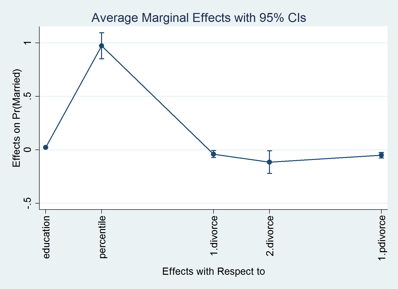
After margins, we can plot the results in the output table simply by typing marginsplot. marginsplot works with the conventional graphics options and the Graph Editor. For the first example above, for instance, I could type
. quietly margins, dydx(*)

. marginsplot, xlabel(, angle(vertical))

  Variables that uniquely identify margins: _deriv
I added the option xlabel(, angle(vertical)) to obtain vertical labels for the horizontal axis. The result is as follows:
Conclusion
I illustrated how to compute, interpret, and graph marginal effects for nonlinear models with interactions of discrete and continuous variables. To interpret interaction effects, I used the concepts of a cross or double derivative and an Expression. I used simulated data and the probit model for my examples. However, what I wrote extends to other nonlinear models.
Appendix
To verify that your expression for the first derivative is correct, you compare it with the statistic computed by margins with the option dydx(variable). For the example in the text:
. margins,
>     expression(normalden(xb())*(_b[percentile] +
>     education*_b[c.education#c.percentile]))

Predictive margins                            Number of obs     =      5,000
Model VCE    : OIM

Expression   : normalden(xb())*(_b[percentile] +
               education*_b[c.education#c.percentile])

----------------------------------------------------------------------------
             |            Delta-method
             |     Margin   Std. Err.      z    P>|z|   [95% Conf. Interval]
-------------+--------------------------------------------------------------
       _cons |   .9873168    .062047    15.91   0.000   .8657069    1.108927
----------------------------------------------------------------------------

. margins, dydx(percentile)

Average marginal effects                      Number of obs     =      5,000
Model VCE    : OIM

Expression   : Pr(married), predict()
dy/dx w.r.t. : percentile

----------------------------------------------------------------------------
             |            Delta-method
             |      dy/dx   Std. Err.      z    P>|z|   [95% Conf. Interval]
-------------+--------------------------------------------------------------
  percentile |   .9873168    .062047    15.91   0.000   .8657069    1.108927
----------------------------------------------------------------------------
Average marginal effect of an interaction between a continuous and a discrete variable as a double derivative:
. margins, expression(normal(_b[education]*education +
>          _b[percentile]*percentile +
>          _b[c.education#c.percentile]*education*percentile +
>          _b[1.divorce#c.education]*education +
>          _b[1.pdivorce]*pdivorce + _b[1.divorce] +
>          _b[1.pdivorce#1.divorce]*1.pdivorce +
>          _b[_cons]) -
>          normal(_b[education]*education +
>          _b[percentile]*percentile +
>          _b[c.education#c.percentile]*education*percentile
>          + _b[1.pdivorce]*pdivorce +
>          _b[_cons])) dydx(education)
Warning: expression() does not contain predict() or xb().

Average marginal effects                      Number of obs     =      5,000
Model VCE    : OIM

Expression   : normal(_b[education]*education + _b[percentile]*percentile +
               _b[c.education#c.percentile]*education*percentile +
               _b[1.divorce#c.education]*education + _b[1.pdivorce]*pdivorce
               + _b[1.divorce] + _b[1.pdivorce#1.divorce]*1.pdivorce +
               _b[_cons]) - normal(_b[education]*education +
               _b[percentile]*percentile +
               _b[c.education#c.percentile]*education*percentile +
               _b[1.pdivorce]*pdivorce + _b[_cons])
dy/dx w.r.t. : education

----------------------------------------------------------------------------
             |            Delta-method
             |      dy/dx   Std. Err.      z    P>|z|   [95% Conf. Interval]
-------------+--------------------------------------------------------------
   education |   .0012968   .0061667     0.21   0.833  -.0107897    .0133833
----------------------------------------------------------------------------
Average marginal effect of an interaction between two continuous variables as a double derivative:
. margins, expression(normalden(xb())*(-xb())*(_b[education]
>       + percentile*_b[c.education#c.percentile] +
>       1.divorce*_b[c.education#1.divorce] +
>       2.divorce*_b[c.education#2.divorce])*(_b[percentile] +
>       education*_b[c.education#c.percentile]) +
>       normalden(xb())*(_b[c.education#c.percentile]))

Predictive margins                            Number of obs     =      5,000
Model VCE    : OIM

Expression   : normalden(xb())*(-xb())*(_b[education] +
               percentile*_b[c.education#c.percentile] +
               1.divorce*_b[c.education#1.divorce] +
               2.divorce*_b[c.education#2.divorce])*(_b[percentile] +
               education*_b[c.education#c.percentile]) +
               normalden(xb())*(_b[c.education#c.percentile])

----------------------------------------------------------------------------
             |            Delta-method
             |     Margin   Std. Err.      z    P>|z|   [95% Conf. Interval]
-------------+--------------------------------------------------------------
       _cons |   .0619111    .021641     2.86   0.004   .0194955    .1043267
----------------------------------------------------------------------------
The simulated data:
clear
set obs 5000
set seed 111
generate education  = int(rbeta(4,2)*15)
generate percentile = int(rbeta(1,7)*100)/100
generate divorce    = int(rbeta(1,4)*3)
generate pdivorce   = runiform()<.6
generate e          = rnormal()
generate xbeta      = .35*(education*.06 + .5*percentile +   ///
                      .8*percentile*education                ///
                      + .07*education*divorce - .5*divorce - ///
                      .2*pdivorce - divorce*pdivorce - .1)
generate married    = xbeta + e > 0