\(\def\bfA{{\bf A}}
\def\bfB{{\bf }}
\def\bfC{{\bf C}}\)Introduction

In this blog post, I describe Stata’s capabilities for estimating and analyzing vector autoregression (VAR) models with long-run restrictions by replicating some of the results of Blanchard and Quah (1989).

Framework

In previous posts, I have identified the parameters of a structural VAR model by imposing restrictions on how shocks influence endogenous variables on impact. By contrast, Blanchard and Quah (1989) achieve identification by imposing restrictions on how shocks influence endogenous variables “in the long run”, that is, the limiting response of an endogenous variable to a shock.

In a stationary VAR, the response of each variable to each shock must be zero in the limit. Blanchard and Quah (1989) analyze a system composed of real gross national product (GNP) and unemployment, where the growth rate of GNP and the level of the unemployment rate are assumed to be stationary. They have two shocks, which they term “supply” and “demand” shocks, and the long-run response of GNP growth and unemployment to those shocks must be zero because these variables are stationary. The identifying restriction is that an impulse to the “demand” shock has no effect on the level of GNP in the long run. Hence, the cumulative response of GNP growth to the demand shock will be constrained to zero. The supply shock is thus defined as that which leads to a long-run change in the level of GNP, and the demand shock is defined as that which does not change the long-run level of GNP.

The Blanchard and Quah (1989) VAR is
\begin{align*}
\bfA(L) \begin{bmatrix} \Delta \mathrm{gnp}_t \\ \mathrm{unrate}_t \end{bmatrix}
=
\bfB \begin{bmatrix} e_t^{\mathrm{supply}} \\ e_t^{\mathrm{demand}} \end{bmatrix}
\end{align*}
where \(L\) is the lag operator and \(\bfA(L)\) is a polynomial lag. We can invert the VAR into
\begin{align*}
\begin{bmatrix} \Delta \mathrm{gnp}_t \\ \mathrm{unrate}_t \end{bmatrix}
=
\bfC(L) \begin{bmatrix} e_t^{\mathrm{supply}} \\ e_t^{\mathrm{demand}} \end{bmatrix}
\end{align*}
The \(\bfC(L)\) matrix is two-by-two and captures the long-run response to shocks. The identification assumption in Blanchard and Quah (1989) is that \(C_{12}=0\), which is equivalent to requiring that the level of GNP eventually return to 0 (or trend) after a shock to the unemployment equation (the “demand” shock).

Data and replication

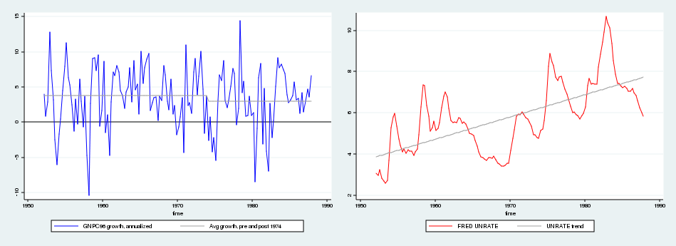
The data for this exercise are found in FRED codes GNPC96 and UNRATE, which I load into Stata using the freduse command; see ssc install freduse. The unemployment rate is measured as the quarterly average of monthly observations on UNRATE. GNP growth is measured as 400 times the log difference in quarterly observations on GNP. Data in the Federal Reserve Economic Database are updated over time because of the addition of new observations and revisions to existing observations, so the data I use will not be identical to those that Blanchard and Quah (1989) used. The dataset I use can be downloaded here.

Blanchard and Quah (1989) use quarterly data from 1952 to 1987, which is shown below. The authors adjust the raw data by removing the mean from GNP growth separately for the pre-1974 and post-1974 subsamples and by removing a linear time trend from the unemployment series.

After loading the raw data, I adjust the unemployment and GNP growth series in line with Blanchard and Quah’s (1989) article.

. use lrsvar.dta

. keep if year >= 1952
(20 observations deleted)

. keep if year <= 1987
(115 observations deleted)

. quietly regress unrate t

. predict unrate_adj, resid

The first three lines load the data and restrict the sample to 1952–1987. The next two lines remove a time trend from the unemployment series and store the residuals into unrate_adj.

Continuing, I adjust the GNP growth series as in Blanchard and Quah (1989).

. generate bp1 = (year<1974)

. generate bp2 = (year>=1974)

. quietly regress growth bp1 bp2, noconstant

. predict growth_adj, resid

The first two lines create dummy variables, one of which equals 1 before the 1974 break point and the other of which equals 1 after the 1974 break point. The final two lines remove the period-specific mean from GNP growth and store the resulting series into growth_adj.

The long-run structural VAR (SVAR) is estimated with svar using the lreq() option. Place GNP growth first in the ordering. Then, the identifying restriction is that the long-run GNP response to the unemployment shock is zero, which leads us to use the restriction matrix C = (.,0 \ .,.). In this matrix, three entries are free (set to missing), and the remaining entry is forced to zero. The authors use eight lags in the VAR, which I follow here. We estimate the SVAR and create impulse–responses with

. matrix C = (., 0 \ .,.)

. svar growth_adj unrate_adj, lags(1/8) lreq(C)
Estimating long-run parameters

Iteration 0:   log likelihood = -1560.8311
Iteration 1:   log likelihood = -419.61266
Iteration 2:   log likelihood = -346.71202
Iteration 3:   log likelihood = -345.55296
Iteration 4:   log likelihood = -345.54985
Iteration 5:   log likelihood = -345.54985

Structural vector autoregression

 ( 1)  [c_1_2]_cons = 0

Sample:  29 - 164                               Number of obs     =        136
Exactly identified model                        Log likelihood    =  -345.5499

------------------------------------------------------------------------------
             |      Coef.   Std. Err.      z    P>|z|     [95% Conf. Interval]
-------------+----------------------------------------------------------------
      /c_1_1 |   1.512693   .0917205    16.49   0.000     1.332924    1.692462
      /c_2_1 |  -.3317345   .3803352    -0.87   0.383    -1.077178    .4137087
      /c_1_2 |          0  (constrained)
      /c_2_2 |   4.429225   .2685612    16.49   0.000     3.902855    4.955595
------------------------------------------------------------------------------

. irf create lr, set(lrirf) step(40) replace
(file lrirf.irf now active)
(file lrirf.irf updated)

I have given the impulse–responses a name, lr, and saved them to a file, lrirf.irf.

We can view the impulse–responses with

. irf graph sirf, yline(0,lcolor(black)) xlabel(0(4)40) byopts(yrescale)
standard errors from all selected results are missing, cannot compute 
    confidence intervals for the chosen statistics

The impulse–responses to each shock under the long-run identification scheme are held in sirf and are graphed in the next figure. One step is one quarter, so the figure depicts the impulse–response over a period of 10 years.

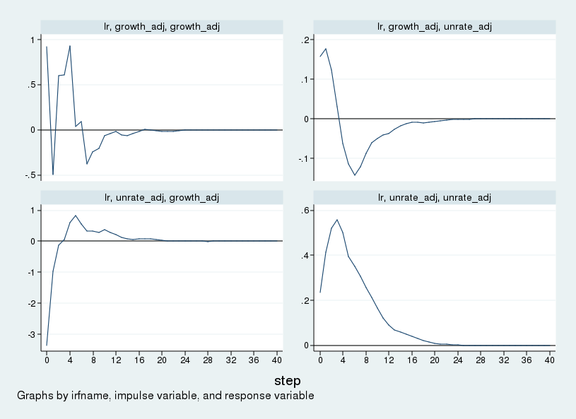
Because GNP growth is ordered first, what Stata calls the "growth impulse" is what Blanchard and Quah (1989) call the "supply" shock. Similarly, the "unrate impulse" is the "demand" shock. The top row shows the response of GNP growth and unemployment to a supply shock. GNP growth rises; the unemployment rate rises on impact, then falls after about one year, troughs after about two years, then slowly returns to its steady-state value. The bottom row shows the response to a "demand" shock. In response to a "demand" shock, output growth falls initially before recovering after one year. Unemployment rises, peaking about a year after the shock before returning to its steady-state value.

Modifying the IRF graph

The impulse–responses in the above figure are in terms of the growth rate of GNP and the level of the unemployment rate, as specified in the SVAR. It is common instead to graph the response of the level of GNP. This involves creating an impulse–response graph that cumulates the response of GNP growth but leaves the response of unemployment unchanged. This section looks inside the .irf file and creates a series that contains the response of the level of GNP and the level of unemployment to shocks. Graphing the response of the level of GNP will also more clearly show the identification assumption we have made.

An .irf file is just a Stata data file with a particular nested panel structure. You can access it with use just like any other dataset, and you can modify it just like any other dataset.

The following code block creates a new variable, csirf, that holds the cumulative impulse–response of GNP growth to each shock and does nothing to the impulse–response to the unemployment rate.

. use lrirf.irf, clear

. sort irfname impulse response step

. gen csirf = sirf

. by irfname impulse: replace csirf = sum(sirf) if response=="growth_adj"
(80 real changes made)

. order irfname impulse response step sirf csirf

. save lrirf2.irf, replace
file lrirf2.irf saved

The first line imports the lrirf.irf dataset into Stata. The second line guarantees that the data are sorted in the correct order: first by irfname, then by the impulse variable, then by the response variable, and finally by step. The third line generates our new variable, csirf, and loads it initially with the values in sirf. The fourth line replaces the values in csirf with the cumulation of values in sirf, but only for the response variable growth_adj, and does so by ifrname and impulse. I save the results to a new irf file, lrirf2.irf. The result is a variable that holds the cumulated response to changes in GNP growth and leaves the responses to unemployment unchanged, which is what we sought.

We can graph the cumulated responses with

. irf set lrirf2.irf
(file lrirf2.irf now active)

. irf graph csirf, yline(0,lcolor(black)) noci xlabel(0(4)40) byopts(yrescale)

and the accompanying graph is in the following figure.

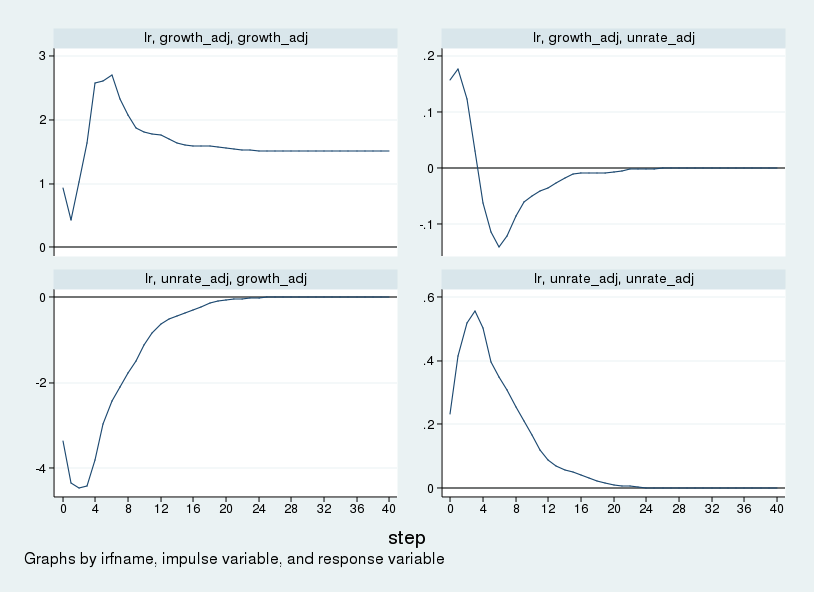
This figure can be compared with figure 1 in Blanchard and Quah (1989). The figures match aside from the scale. Differences in the scale of the impulse–responses are due to differences in the size of the initial impulse. Stata uses a one-standard-deviation impulse, while Blanchard and Quah (1989) use a one-unit impulse. In the top-left panel we see that the supply shock increases the level of GNP permanently. In the bottom-left panel, we see that GNP falls in response to a demand shock but returns to zero (or trend) over time. The long-run zero response in the bottom-left panel visually displays our identification assumption.

Conclusion

In this post, I outlined a procedure to estimate a SVAR with long-run restrictions and showed how to modify the resulting IRF file to contain a series that displays cumulative structural impulse–responses for some variables in the VAR.

Reference

Blanchard, O. J. and D. Quah. 1989. The dynamic effects of aggregate demand and supply disturbances. American Economic Review 79: 655–673.