Understanding truncation and censoring
Truncation and censoring are two distinct phenomena that cause our samples to be incomplete. These phenomena arise in medical sciences, engineering, social sciences, and other research fields. If we ignore truncation or censoring when analyzing our data, our estimates of population parameters will be inconsistent.
Truncation or censoring happens during the sampling process. Let’s begin by defining left-truncation and left-censoring:
Our data are left-truncated when individuals below a threshold are not present in the sample. For example, if we want to study the size of certain fish based on the specimens captured with a net, fish smaller than the net grid won’t be present in our sample.
Our data are left-censored at \(\kappa\) if every individual with a value below \(\kappa\) is present in the sample, but the actual value is unknown. This happens, for example, when we have a measuring instrument that cannot detect values below a certain level.
We will focus our discussion on left-truncation and left-censoring, but the concepts we will discuss generalize to all types of censoring and truncation—right, left, and interval.
When performing estimations with truncated or censored data, we need to use tools that account for that type of incomplete data. For truncated linear regression, we can use the truncreg command, and for censored linear regression, we can use the intreg or tobit command.
In this blog post, we will analyze the characteristics of truncated and censored data and discuss using truncreg and tobit to account for the incomplete data.
Truncated data
Example: Royal Marines
Fogel et al. (1978) published a dataset on the height of Royal Marines that extends over two centuries. It can be used to determine the mean height of men in Britain for different periods of time. Trussell and Bloom (1979) point out that the sample is truncated due to minimum height restrictions for the recruits. The data are truncated (as opposed to censored) because individuals with heights below the minimum allowed height do not appear in the sample at all. To account for this fact, they fit a truncated distribution to the heights of Royal Marines from the period 1800–1809.
We are using an artificial dataset based on the problem described by Trussell and Bloom. We’ll assume that the population data follow a normal distribution with \(\mu=65\) and \(\sigma=3.5\), and that they are left-truncated at 64.
We use a histogram to summarize our data.
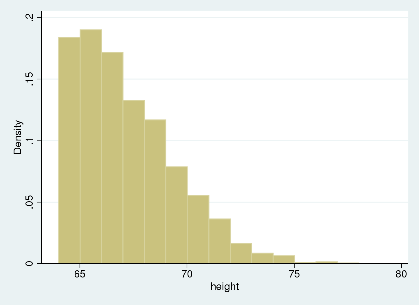
We see there are no data below 64, our truncation point.
What happens if we ignore truncation?
If we ignore the truncation and treat the incomplete data as complete, the sample average is inconsistent for the population mean, because all observations below the truncation point are missing. In our example, the true mean is outside the 95% confidence interval for
the estimated mean.
. mean height

Mean estimation                   Number of obs   =      2,200

--------------------------------------------------------------
             |       Mean   Std. Err.     [95% Conf. Interval]
-------------+------------------------------------------------
      height |   67.18388   .0489487      67.08788    67.27987
--------------------------------------------------------------

. estat sd

-------------------------------------
             |       Mean   Std. Dev.
-------------+-----------------------
      height |   67.18388    2.295898
-------------------------------------
We can compare the histogram of our sample to the normal distribution that we get if we ignore truncation, and consider these values as estimates of the mean and standard deviation of the population.
. histogram height , width(1)
>         addplot( function f1 = normalden(x, 67.18, 2.30), range(55 75))
(bin=14, start=64.017105, width=1)
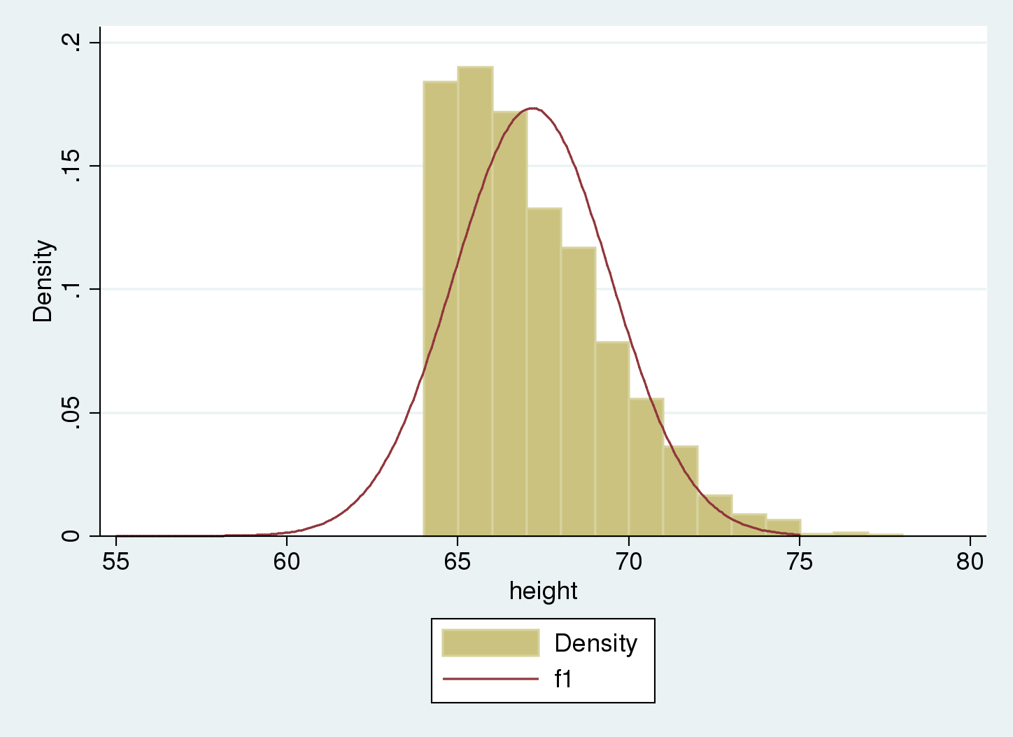
We see that the Gaussian density estimate, \(f_1\), which ignored truncation, is shifted to the right of the histogram, and the variance seems to be underestimated. We can verify this because we used artificial data that were simulated with an underlying mean of 65 and standard deviation of 3.5 for the nontruncated distribution, as opposed to the estimated mean of 67.2 and standard deviation of 2.3.
Using truncreg to account for truncation
We can use truncreg to estimate the parameters for the underlying nontruncated distribution; to account for the left-truncation at 64, we use option ll(64).
. truncreg height, ll(64)
(note: 0 obs. truncated)

Fitting full model:

Iteration 0:   log likelihood = -4759.5965
Iteration 1:   log likelihood =  -4603.043
Iteration 2:   log likelihood = -4600.5217
Iteration 3:   log likelihood = -4600.4862
Iteration 4:   log likelihood = -4600.4862

Truncated regression
Limit:   lower =         64                     Number of obs     =      2,200
         upper =       +inf                     Wald chi2(0)      =          .
Log likelihood = -4600.4862                     Prob > chi2       =          .

------------------------------------------------------------------------------
      height |      Coef.   Std. Err.      z    P>|z|     [95% Conf. Interval]
-------------+----------------------------------------------------------------
       _cons |   64.97701   .2656511   244.60   0.000     64.45634    65.49768
-------------+----------------------------------------------------------------
      /sigma |   3.506442   .1303335    26.90   0.000     3.250993    3.761891
------------------------------------------------------------------------------
Now, estimates are close to our actual simulated values, \(\mu = 65\), \(\sigma=3.5\).
Let’s overlap the truncated density to the data histogram.
. histogram height , width(1)
>   addplot(function f_trunc =
>   cond(x<64, 0, normalden(x, 64.97, 3.51)/(1-normal((64-64.97)/3.51))),
>   range(55 75))
(bin=14, start=64.017105, width=1)
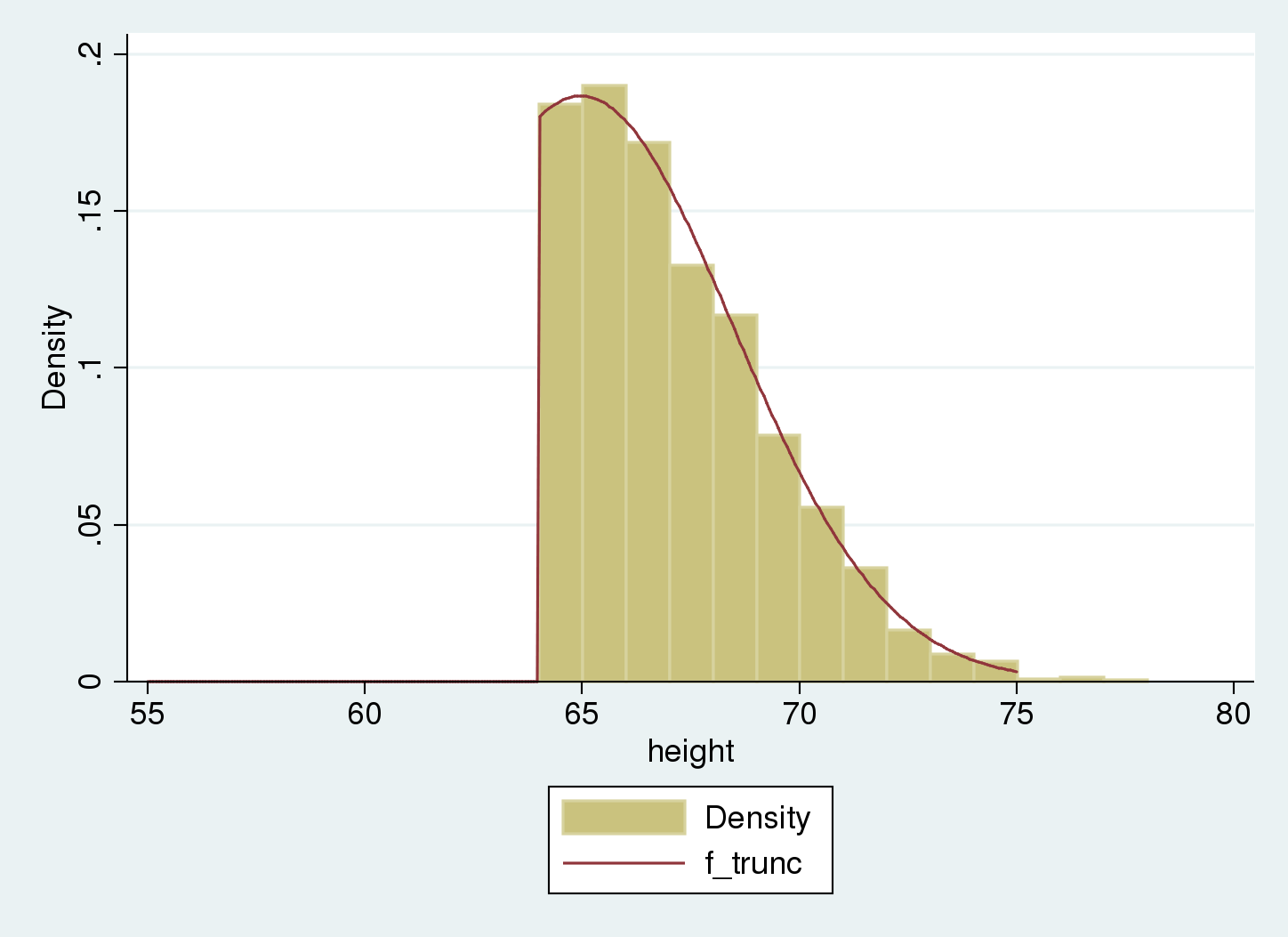
The truncated distribution fits our sample. We estimate the population distribution as normal with mean equal to 65 and standard deviation equal to 3.5.
Censored data
Now we consider an example with censored data rather than truncated data to demonstrate the difference between the two.
Example: Nicotine levels on household surfaces
Matt et al. (2004) performed a study to assess contamination with tobacco smoke on surfaces in households of smokers. One measurement of interest was the level of nicotine on furniture surfaces. For each household, area wipe samples were taken from the furniture. However, the measurement instrument could not detect nicotine contamination below a certain limit.
The data were censored as opposed to truncated. When the nicotine level fell below the detection limit, the observation was still included in the sample with the nicotine level recorded as being equal to that limit.
I have created an artificial dataset loosely inspired by the problem in this study. The log of nicotine contamination levels are assumed to be normal. Here, lognlevel contains log nicotine levels. The parameters used for simulating the log nicotine levels for uncensored data are \(\mu=\ln(5)\) and \(\sigma=2.5\), and the data have been left-censored at 0.1. We start by drawing a histogram.
. histogram lognlevel, width(.25)
(bin=53, start=-2.3025851, width=.25)
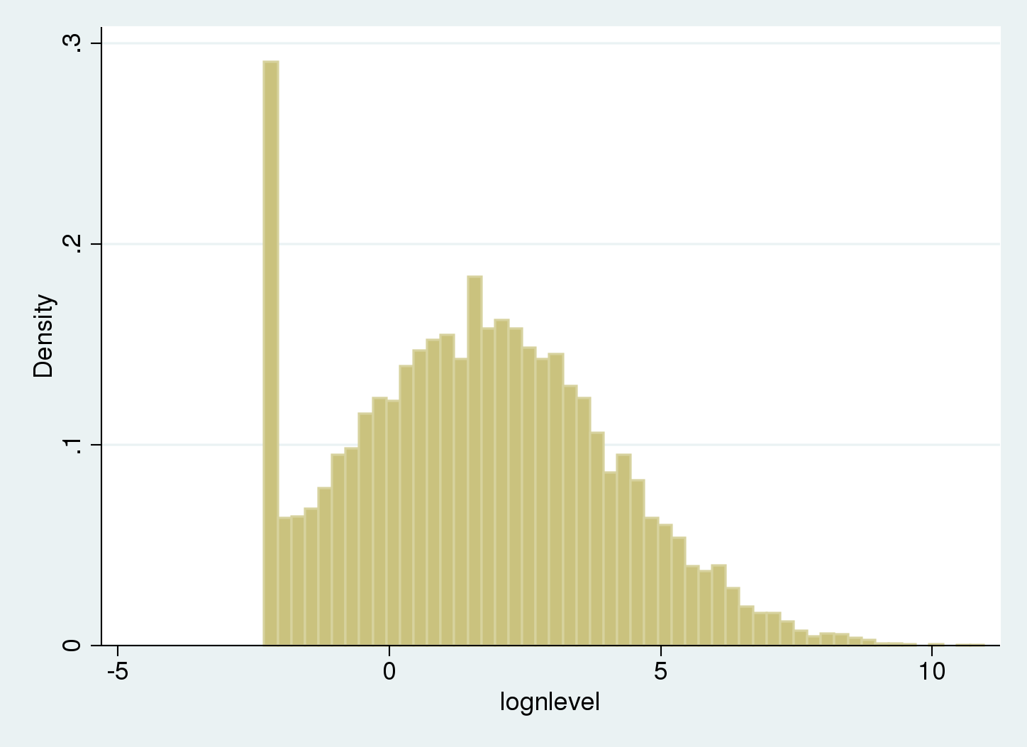
There is a spike on the left of the histogram because values below the limit of detection (LOD) are recorded as being equal to the LOD.
Computing the raw mean and standard deviation for the sample will not provide appropriate estimates for the underlying uncensored Gaussian distribution.
. summarize lognlevel

    Variable |        Obs        Mean    Std. Dev.       Min        Max
-------------+---------------------------------------------------------
   lognlevel |     10,000    1.683339    2.360516  -2.302585   10.73322
Mean and standard deviation are estimated as 1.68 and 2.4 respectively, where the actual parameters are ln(5) =1.61 and 2.5.
Using tobit to account for censoring
We estimate the mean and standard deviation of the distribution and account for the left-censoring by using tobit with the ll option. (If censoring limits varied among observations, we could use intreg instead).
. tobit lognlevel, ll

Tobit regression                                Number of obs     =     10,000
                                                LR chi2(0)        =       0.00
                                                Prob > chi2       =          .
Log likelihood = -22680.512                     Pseudo R2         =     0.0000

------------------------------------------------------------------------------
   lognlevel |      Coef.   Std. Err.      t    P>|t|     [95% Conf. Interval]
-------------+----------------------------------------------------------------
       _cons |   1.620857   .0249836    64.88   0.000     1.571884     1.66983
-------------+----------------------------------------------------------------
      /sigma |   2.486796   .0184318                      2.450666    2.522926
------------------------------------------------------------------------------
           588  left-censored observations at lognlevel <= -2.3025851
         9,412     uncensored observations
             0 right-censored observations
The underlying uncensored distribution is estimated as normal with mean 1.62 and standard deviation 2.49.
Let's overlap the uncensored distribution to the histogram:
. histogram lognlevel , width(.25)
>  addplot( function f = normalden(x, 1.62, 2.49), range(-5 10))
(bin=53, start=-2.3025851, width=.25)
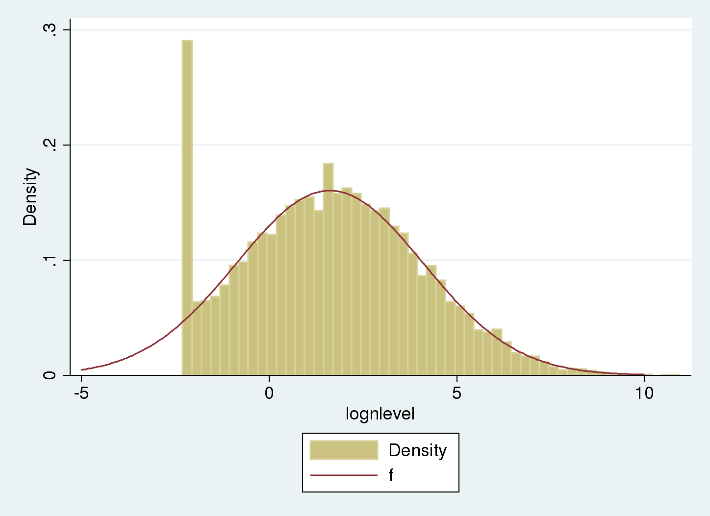
The underlying uncensored distribution matches the regular part of the histogram. The tail on the left compensates the spike at the censoring point.
Summary
Censoring and truncation are two distinct phenomena that happen when sampling data.
The underlying population parameters for a truncated Gaussian sample can be estimated with truncreg. The underlying population parameters for a censored Gaussian sample can be estimated with intreg or tobit.
Final remarks
We've discussed the concepts of censoring and truncation, and shown examples to illustrate those concepts.
There are some relevant points related to this discussion that I would like to point out:
The discussion above is based on the Gaussian model, but the main concepts extend to any distribution.
The examples above fit regression models without covariates, so we can better visualize the shape of the censored and truncated distributions. However, these concepts are easily extended to a regression framework with covariates where the expected value of a particular observation is a function of the covariates.
I have discussed the use of truncreg and tobit for censored and truncated data. However, those commands can also be applied to data that are not truncated or censored but that are sampled from a population with certain specific distributions.
References
Fogel, R. W., S. L. Engerman, J. Trussell, R. Floud, C. L. Pope and L. T. Wimmer. 1978.
The economics of mortality in North America, 1650–1910: A description of a research project. Historical Methods 11: 75–108.
Matt, G. E., P. J. E. Quintana, M. F. Hovell, J. T. Bernert, S. Song, N. Novianti, T. Juarez, J. Floro, C. Gehrman, M. Garcia, S. Larson. 2004. Households contaminated by environmental tobacco smoke: sources of infant exposures. Tobacco Control 13: 27–29.
Trussell, J. and D. E. Bloom. 1979. A model distribution of height or weight at a given age. Human Biology 51: 523–536.