Introduction

Dynamic stochastic general equilibrium (DSGE) models are used in macroeconomics to model the joint behavior of aggregate time series like inflation, interest rates, and unemployment. They are used to analyze policy, for example, to answer the question, “What is the effect of a surprise rise in interest rates on inflation and output?” To answer that question we need a model of the relationship among interest rates, inflation, and output. DSGE models are distinguished from other models of multiple time series by their close connection to economic theory. Macroeconomic theories consist of systems of equations that are derived from models of the decisions of households, firms, policymakers, and other agents. These equations form the DSGE model. Because the DSGE model is derived from theory, its parameters can be interpreted directly in terms of the theory.

In this post, I build a small DSGE model that is similar to models used for monetary policy analysis. I show how to estimate the parameters of this model using the new dsge command in Stata 15. I then shock the model with a contraction in monetary policy and graph the response of model variables to the shock.

A small DSGE model

A DSGE model begins with a description of the sectors of the economy to be modeled. The model I describe here is related to the models developed in Clarida, Galí, and Gertler (1999) and Woodford (2003). It is a smaller version of the kinds of models used in central banks and academia for monetary policy analysis. The model has three sectors: households, firms, and a central bank.

• Households consume output. Their decision making is summarized by an output demand equation that relates current output demand to expected future output demand and the real interest rate.
• Firms set prices and produce output to satisfy demand at the set price. Their decision making is summarized by a pricing equation that relates current inflation (that is, the change in prices) to expected future inflation and current demand. The parameter capturing the degree to which inflation depends on output demand plays a key role in the model.
• The central bank sets the nominal interest rate in response to inflation. The central bank increases the interest rate when inflation rises and reduces the interest rate when inflation falls.

The model can be summarized in three equations,
\begin{align}
x_t &= E_t(x_{t+1}) – \{r_t – E_t(\pi_{t+1}) – z_t\} \\
\pi_t &= \beta E_t(\pi_{t+1}) + \kappa x_t \\
r_t &= \frac{1}{\beta} \pi_t + u_t
\end{align}

The variable \(x_t\) denotes the output gap. The output gap measures the difference between output and its long run, natural value. The notation \(E_t(x_{t+1})\) specifies the expectation, conditional on information available at time \(t\), of the output gap in period \(t+1\). The nominal interest rate is \(r_t\), and the inflation rate is \(\pi_t\). Equation (1) states that the output gap is related positively to the expected future output gap, \(E_t(x_{t+1})\), and negatively to the interest rate gap, \(\{r_t – E_t(\pi_{t+1}) – z_t\}\). The second equation is the firm’s pricing equation; it relates inflation to expected future inflation and the output gap. The parameter \(\kappa\) determines the extent to which inflation depends on the output gap. Finally, the third equation summarizes the central bank’s behavior; it relates the interest rate to inflation and to other factors, collectively termed \(u_t\).

The endogenous variables \(x_t\), \(\pi_t\), and \(r_t\) are driven by two exogenous variables, \(z_t\) and \(u_t\). In terms of the theory, \(z_t\) is the natural rate of interest. If the real interest rate is equal to the natural rate and is expected to remain so in the future, then the output gap is zero. The exogenous variable \(u_t\) captures all movements in the interest rate that arise from factors other than movements in inflation. It is sometimes referred to as the surprise component of monetary policy.

The two exogenous variables are modeled as first-order autoregressive processes,
\begin{align}
z_{t+1} &= \rho_z z_t + \varepsilon_{t+1} \\
u_{t+1} &= \rho_u u_t + \xi_{t+1}
\end{align}
which follows common practice.

In the jargon, endogenous variables are called control variables, and exogenous variables are called state variables. The values of control variables in a period are determined by the system of equations. Control variables can be observed or unobserved. State variables are fixed at the beginning of a period and are unobserved. The system of equations determines the value of state variables one period in the future.

We wish to use the model to answer policy questions. What is the effect on model variables when the central bank conducts a surprise increase in the interest rate? The answer to this question is to impose an impulse \(\xi_t\) and trace out the effect of the impulse over time.

Before doing policy analysis, we must assign values to the parameters of the model. We will estimate the parameters of the above model using U.S. data on inflation and interest rates with dsge in Stata.

Specifying the DSGE to dsge

I fit the model using data on the U.S. interest rate and inflation rate. In a DSGE model, you can have as many observable control variables as you have shocks in the model. Because the model has two shocks, we have two observable control variables. The variables in a linearized DSGE model are stationary and measured in deviation from steady state. In practice, this means the data must be de-meaned prior to estimation. dsge will remove the mean for you.

I use the data in usmacro2, which is drawn from the Federal Reserve Bank of St. Louis database.

. webuse usmacro2

To specify a model to Stata, type the equations using substitutable expressions.

. dsge (x = E(F.x) - (r - E(F.p) - z), unobserved) ///
       (p = {beta}*E(F.p) + {kappa}*x)             ///
       (r = 1/{beta}*p + u)                        ///
       (F.z = {rhoz}*z, state)                     ///
       (F.u = {rhou}*u, state)

The rules for equations are similar to those for Stata’s other commands that work with substitutable expressions. Each equation is bound in parentheses. Parameters are enclosed in braces to distinguish them from variables. Expectations of future variables appear within the E() operator. One variable appears on the left-hand side of the equation. Further, each variable in the model appears on the left-hand side of one and only one equation. Variables can be either observed (exist as variables in your dataset) or unobserved. Because the state variables are fixed in the current period, equations for state variables express how the one-step-ahead value of the state variable depends on current state variables and, possibly, current control variables.

Estimating the model parameters gives us an output table:

. dsge (x = E(F.x) - (r - E(F.p) - z), unobserved) ///
>      (p = {beta}*E(F.p) + {kappa}*x)             ///
>      (r = 1/{beta}*p + u)                        ///
>      (F.z = {rhoz}*z, state)                     ///
>      (F.u = {rhou}*u, state)
(setting technique to bfgs)
Iteration 0:   log likelihood = -13738.863
Iteration 1:   log likelihood = -1311.9615  (backed up)
Iteration 2:   log likelihood = -1024.7903  (backed up)
Iteration 3:   log likelihood = -869.19312  (backed up)
Iteration 4:   log likelihood = -841.79194  (backed up)
(switching technique to nr)
Iteration 5:   log likelihood =  -819.0268  (not concave)
Iteration 6:   log likelihood =  -782.4525  (not concave)
Iteration 7:   log likelihood = -764.07067
Iteration 8:   log likelihood = -757.85496
Iteration 9:   log likelihood = -754.02921
Iteration 10:  log likelihood = -753.58072
Iteration 11:  log likelihood = -753.57136
Iteration 12:  log likelihood = -753.57131

DSGE model

Sample: 1955q1 - 2015q4                         Number of obs     =        244
Log likelihood = -753.57131
------------------------------------------------------------------------------
             |                 OIM
             |      Coef.   Std. Err.      z    P>|z|     [95% Conf. Interval]
-------------+----------------------------------------------------------------
/structural  |
        beta |    .514668    .078349     6.57   0.000     .3611067    .6682292
       kappa |   .1659046    .047407     3.50   0.000     .0729885    .2588207
        rhoz |   .9545256   .0186424    51.20   0.000     .9179872     .991064
        rhou |   .7005492   .0452603    15.48   0.000     .6118406    .7892578
-------------+----------------------------------------------------------------
      sd(e.z)|   .6211208   .1015081                      .4221685     .820073
      sd(e.u)|     2.3182   .3047433                      1.720914    2.915486
------------------------------------------------------------------------------

The crucial parameter is {kappa}, which is estimated to be positive. This parameter is related to the underlying price frictions in the model. Its interpretation is that if we hold expected future inflation constant, a 1 percentage point increase in the output gap leads to a 0.17 percentage point increase in inflation.

The parameter \(\beta\) is estimated to be about 0.5, meaning that the coefficient on inflation in the interest rate equation is about 2. So the central bank increases the interest rate about two for one in response to movements in inflation. This parameter is much discussed in the monetary economics literature, and estimates of it cluster around 1.5. The value found here is comparable with those estimates. Both state variables \(z_t\) and \(u_t\) are estimated to be persistent, with autoregressive coefficients of 0.95 and 0.7, respectively.

Impulse–responses

We can now use the model to answer questions. One question the model can answer is, “What is the effect of an unexpected change in the interest rate on inflation and the output gap?” An unexpected change in the interest rate is modeled as a shock to the \(u_t\) equation. In the language of the model, this shock represents a contraction in monetary policy.

An impulse is a series of values for the shock \(\xi\) in (5): \((1, 0, 0, 0, 0, \dots)\). The shock then feeds into the model’s state variables, leading to an increase in \(u\). From there, the increase in \(u\) leads to a change in all the model’s control variables. An impulse–response function traces out the effect of a shock on the model variables, taking into account all the interrelationships among variables present in the model equations.

We type three commands to build and graph an IRF. irf set sets the IRF file that will hold the impulse–responses. irf create creates a set of impulse–responses in the IRF file.

. irf set dsge_irf
. irf create model1

With the impulse–responses saved, we can graph them:

. irf graph irf, impulse(u) response(x p r u) byopts(yrescale) yline(0)

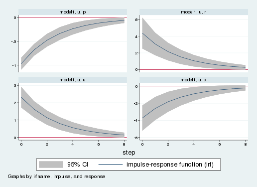
The impulse–response graphs the response of model variables to a one-standard-deviation shock. Each panel is the response of one variable to the shock. The horizontal axis measures time since the shock, and the vertical axis measures deviations from long-run value. The bottom-left panel shows the response of the monetary state variable, \(u_t\). The remaining three panels show the response of inflation, the interest rate, and the output gap. Inflation is in the top-left panel; it falls on impact of the shock. The interest rate response in the upper-right panel is a weighted sum of the inflation and monetary impulse–responses. The interest rate rises by about one-half of one percentage point. Finally, the output gap falls. Hence, the model predicts that after a monetary tightening, the economy will enter a recession. Over time, the effect of the shock dissipates, and all variables return to their long-run values.

Conclusion

In this post, I developed a small DSGE model and described how to estimate the parameters of the model using dsge. I then showed how to create and interpret an impulse–response function.

References

Clarida, R., J. Galí, and M. Gertler. 1999. The science of monetary policy: A new Keynesian perspective. Journal of Economic Literature 37: 1661–1707.

Woodford, M. 2003. Interest and Prices: Foundations of a Theory of Monetary Policy. Princeton, NJ: Princeton University Press.