Bayesian logistic regression with Cauchy priors using the bayes prefix
Introduction
Stata 15 provides a convenient and elegant way of fitting Bayesian regression models by simply prefixing the estimation command with bayes. You can choose from 45 supported estimation commands. All of Stata’s existing Bayesian features are supported by the new bayes prefix. You can use default priors for model parameters or select from many prior distributions. I will demonstrate the use of the bayes prefix for fitting a Bayesian logistic regression model and explore the use of Cauchy priors (available as of the update on July 20, 2017) for regression coefficients.
A common problem for Bayesian practitioners is the choice of priors for the coefficients of a regression model. The conservative approach of specifying very weak or completely uninformative priors is considered to be data-driven and objective, but is at odds with the Bayesian paradigm. Noninformative priors may also be insufficient for resolving some common regression problems such as the separation problem in logistic regression. On the other hand, in the absence of strong prior knowledge, there are no general rules for choosing informative priors. In this article, I follow some recommendations from Gelman et al. (2008) for providing weakly informative Cauchy priors for the coefficients of logistic regression models and demonstrate how these priors can be specified using the bayes prefix command.
Data
I consider a version of the well known Iris dataset (Fisher 1936) that describes three iris plants using their sepal and petal shapes. The binary variable virg distinguishes the Iris virginica class from those of Iris Versicolour and Iris Setosa. The variables slen and swid describe sepal length and width. The variables plen and pwid describe petal length and width. These four variables are standardized, so they have mean 0 and standard deviation 0.5.
Standardizing the variables used as covariates in a regression model is recommended by Gelman et al. (2008) to apply common prior distributions to the regression coefficients. This approach is also favored by other researchers, for example, Raftery (1996).
. use irisstd

. summarize

    Variable |        Obs        Mean    Std. Dev.       Min        Max
-------------+---------------------------------------------------------
        virg |        150    .3333333    .4729838          0          1
        slen |        150    4.09e-09          .5  -.9318901   1.241849
        swid |        150   -2.88e-09          .5  -1.215422   1.552142
        plen |        150    2.05e-10          .5  -.7817487   .8901885
        pwid |        150    4.27e-09          .5  -.7198134   .8525946
For validation purposes, I withhold the first and last observations from being used in model estimation. I generate the indicator variable touse that will mark the estimation subsample.
. generate touse = _n>1 & _n<_N
Models
I first run a standard logistic regression model with outcome variable virg and predictors slen, swid, plen, and pwid.
. logit virg slen swid plen pwid if touse, nolog

Logistic regression                             Number of obs     =        148
                                                LR chi2(4)        =     176.09
                                                Prob > chi2       =     0.0000
Log likelihood = -5.9258976                     Pseudo R2         =     0.9369

------------------------------------------------------------------------------
        virg |      Coef.   Std. Err.      z    P>|z|     [95% Conf. Interval]
-------------+----------------------------------------------------------------
        slen |  -3.993255   3.953552    -1.01   0.312    -11.74207    3.755564
        swid |  -5.760794   3.849978    -1.50   0.135    -13.30661    1.785024
        plen |   32.73222   16.62764     1.97   0.049     .1426454     65.3218
        pwid |   27.60757   14.78357     1.87   0.062    -1.367681    56.58283
       _cons |  -19.83216   9.261786    -2.14   0.032    -37.98493   -1.679393
------------------------------------------------------------------------------
Note: 54 failures and 6 successes completely determined.
The logit command issues a note that some observations are completely determined. This is due to the fact that the continuous covariates, especially pwid, have many repeating values.
I then fit a Bayesian logistic regression model by prefixing the above command with bayes. I also specify a random-number seed for reproducibility.
. set seed 15

. bayes: logit virg slen swid plen pwid if touse

Burn-in ...
Simulation ...

Model summary
------------------------------------------------------------------------------
Likelihood:
  virg ~ logit(xb_virg)

Prior:
  {virg:slen swid plen pwid _cons} ~ normal(0,10000)                       (1)
------------------------------------------------------------------------------
(1) Parameters are elements of the linear form xb_virg.

Bayesian logistic regression                     MCMC iterations  =     12,500
Random-walk Metropolis-Hastings sampling         Burn-in          =      2,500
                                                 MCMC sample size =     10,000
                                                 Number of obs    =        148
                                                 Acceptance rate  =      .1511
                                                 Efficiency:  min =      .0119
                                                              avg =      .0204
Log marginal likelihood =  -20.64697                          max =     .03992

------------------------------------------------------------------------------
             |                                                Equal-tailed
        virg |      Mean   Std. Dev.     MCSE     Median  [95% Cred. Interval]
-------------+----------------------------------------------------------------
        slen | -7.391316   5.256959   .263113  -6.861438  -18.87585   2.036088
        swid | -9.686068    5.47113   .492419  -9.062651  -21.32787  -1.430718
        plen |  59.90382   23.97788   1.53277   56.48103   23.00752   116.0312
        pwid |  45.65266    22.2054   2.03525   42.01611   14.29399   99.51405
       _cons | -34.50204   13.77856   1.19136  -32.61649  -66.09916  -14.83324
------------------------------------------------------------------------------
Note: Default priors are used for model parameters.
By default, normal priors with mean 0 and standard deviation 100 are used for the intercept and regression coefficients. Default normal priors are provided for convenience, so users can see the naming conventions for parameters to specify their own priors. The chosen priors are selected to be fairly uninformative but may not be so for parameters with large values.
The bayes:logit command produces estimates that are much
higher in absolute value than the corresponding maximum likelihood estimates. For example, the posterior mean estimate for the coefficient of the plen variable, {virg:plen}, is about 60. This means that a unit change in plen results in a 60-unit change for the outcome in the logistic scale, which is very large. The corresponding maximum likelihood estimate is about 33. Given that the default priors are vague, can we explain this difference? Let's look at the sample posterior distribution of the regression coefficients. I draw histograms using the bayesgraph histogram command:
. bayesgraph histogram _all, combine(rows(3))
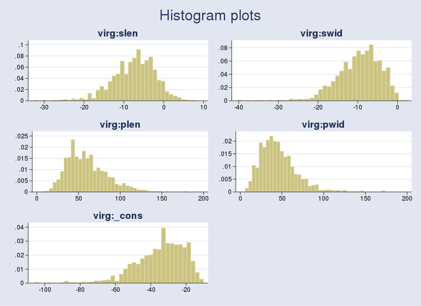
Under vague priors, posterior modes are expected to be close to MLEs. All posterior distributions are skewed. Thus, all sample posterior means are much larger than posterior modes in absolute value and are different from MLEs.
Gelman et al. (2008) suggest applying Cauchy priors for the regression coefficients when data are standardized so that all continuous variables have standard deviation 0.5. Specifically, we use a scale of 10 for the intercept and a scale of 2.5 for the regression coefficients. This choice is based on the observation that within the unit change of each predictor, an outcome change of 5 units on the logistic scale will move the outcome probability from 0.01 to 0.5 and from 0.5 to 0.99.
The Cauchy priors are centered at 0, because the covariates are centered at 0.
. set seed 15

. bayes, prior({virg:_cons}, cauchy(0, 10))                  ///
>         prior({virg:slen swid plen pwid}, cauchy(0, 2.5)): ///
>         logit virg slen swid plen pwid if touse

Burn-in ...
Simulation ...

Model summary
------------------------------------------------------------------------------
Likelihood:
  virg ~ logit(xb_virg)

Priors:
                {virg:_cons} ~ cauchy(0,10)                                (1)
  {virg:slen swid plen pwid} ~ cauchy(0,2.5)                               (1)
------------------------------------------------------------------------------
(1) Parameters are elements of the linear form xb_virg.

Bayesian logistic regression                     MCMC iterations  =     12,500
Random-walk Metropolis-Hastings sampling         Burn-in          =      2,500
                                                 MCMC sample size =     10,000
                                                 Number of obs    =        148
                                                 Acceptance rate  =      .2072
                                                 Efficiency:  min =     .01907
                                                              avg =     .02489
Log marginal likelihood = -18.651475                          max =     .03497

------------------------------------------------------------------------------
             |                                                Equal-tailed
        virg |      Mean   Std. Dev.     MCSE     Median  [95% Cred. Interval]
-------------+----------------------------------------------------------------
        slen |  -2.04014   2.332062   .143792  -1.735382  -7.484299    1.63583
        swid |  -2.59423    2.00863   .107406  -2.351623  -7.379954   .6207466
        plen |  21.27293   10.37093   .717317   19.99503   4.803869   45.14316
        pwid |  16.74598   7.506278    .54353   16.00158   4.382826   35.00463
       _cons | -11.96009   4.157192   .272998  -11.20163  -22.45385  -6.549506
------------------------------------------------------------------------------
We can use bayesgraph diagnostics to verify that there are no convergence problems with the model, but I skip this step here.
The posterior mean estimates in this model are about three times smaller in absolute value than those of the model with default vague normal priors and are closer to the maximum likelihood estimates. For example, the posterior mean estimate for {virg:plen} is now only about 21.
The estimated log-marginal likelihood of the model, -18.7, is higher than that of the model with default normal priors, -20.6, which indicates that the model with independent Cauchy priors fits the data better.
Predictions
Now that we are satisfied with our model, we can perform some postestimation. All Bayesian postestimation features work after the bayes prefix just as they do after the bayesmh command. Below, I show examples of obtaining out-of-sample predictions. Say we want to make predictions for the first and last observations in our dataset, which were not used for fitting the model. The first observation is not from the Iris virginica class, but the last one is.
. list if !touse

     +------------------------------------------------------------+
     | virg       slen        swid       plen        pwid   touse |
     |------------------------------------------------------------|
  1. |    0   -.448837    .5143057   -.668397   -.6542964       0 |
150. |    1   .0342163   -.0622702   .3801059    .3939755       0 |
     +------------------------------------------------------------+
We can use the bayesstats summary command to predict the outcome class by applying the invlogit() transformation to the desired linear combination of predictors.
. bayesstats summary (prob0:invlogit(-.448837*{virg:slen}  ///
>         +.5143057*{virg:swid}-.668397*{virg:plen}        ///
>         -.6542964*{virg:pwid}+{virg:_cons})), nolegend

Posterior summary statistics                      MCMC sample size =    10,000

------------------------------------------------------------------------------
             |                                                Equal-tailed
             |      Mean   Std. Dev.     MCSE     Median  [95% Cred. Interval]
-------------+----------------------------------------------------------------
       prob0 |  7.26e-10   1.02e-08   3.1e-10   4.95e-16   3.18e-31   8.53e-10
------------------------------------------------------------------------------

. bayesstats summary (prob1:invlogit(.0342163*{virg:slen}  ///
>         -.0622702*{virg:swid}+.3801059*{virg:plen}       ///
>         +.3939755*{virg:pwid}+{virg:_cons})), nolegend

Posterior summary statistics                      MCMC sample size =    10,000

------------------------------------------------------------------------------
             |                                                Equal-tailed
             |      Mean   Std. Dev.     MCSE     Median  [95% Cred. Interval]
-------------+----------------------------------------------------------------
       prob1 |  .9135251   .0779741   .004257   .9361961   .7067089   .9959991
------------------------------------------------------------------------------
The posterior mean probability for the first observation to belong to the class Iris virginica is estimated to be essentially zero, 7.3e-10. In contrast, the estimated probability for the last observation is about 0.91. Both predictions agree with the observed classes.
The dataset used in this post is available here: irisstd.dta
References
Gelman, A., A. Jakulin, M. G. Pittau, and Y.-S. Su. 2008. A weakly informative default prior distribution for logistic and other regression models. Annals of Applied Statistics 2: 1360–1383.
Fisher, R. A. 1936. The use of multiple measurements in taxonomic problems. Annals of Eugenics 7: 179–188.
Raftery, A. E. 1996. Approximate Bayes factors and accounting for model uncertainty in generalized linear models. Biometrika 83: 251–266.