Dynamic stochastic general equilibrium models for policy analysis
What are DSGE models?
Dynamic stochastic general equilibrium (DSGE) models are used by macroeconomists to model multiple time series. A DSGE model is based on economic theory. A theory will have equations for how individuals or sectors in the economy behave and how the sectors interact. What emerges is a system of equations whose parameters can be linked back to the decisions of economic actors. In many economic theories, individuals take actions based partly on the values they expect variables to take in the future, not just on the values those variables take in the current period. The strength of DSGE models is that they incorporate these expectations explicitly, unlike other models of multiple time series.
DSGE models are often used in the analysis of shocks or counterfactuals. A researcher might subject the model economy to an unexpected change in policy or the environment and see how variables respond. For example, what is the effect of an unexpected rise in interest rates on output? Or a researcher might compare the responses of economic variables with different policy regimes. For example, a model might be used to compare outcomes under a high-tax versus a low-tax regime. A researcher would explore the behavior of the model under different settings for tax rate parameters, holding other parameters constant.
In this post, I show you how to estimate the parameters of a DSGE model, how to create and interpret an impulse response, and how to compare the impulse response estimated from the data with an impulse response generated by a counterfactual policy regime.
Estimate model parameters
I have monthly data on the growth rate of industrial production and interest rates. I will use these data to estimate the parameters of a small DSGE model. My model has just two agents: firms that produce output (ip) and a central bank that sets interest rates (r). In my model, industrial production growth depends on the expected interest rate one period in the future and on other exogenous factors. In turn, the interest rate depends on contemporaneous industrial production growth and on other latent factors. I call the latent factors affecting production e and the latent factors affecting interest rates m.
The latent factors are known as “state variables” in the jargon. We can impose a shock to state variables and trace out how that shock affects the system. I specify the evolution of m as an AR(1) process. To give the model some additional dynamics, I specify the evolution of e as an AR(2) process. My full model is
\begin{align}\label{eq:fullmodel}
ip_t &= \alpha E(r_{t+1}) + e_t \tag{1}\\
r_t &= \beta ip_t + m_t \tag{2}\\
m_{t+1} &= \rho m_t + v_{t+1} \tag{3}\\
e_{t+1} &= \theta_{1} e_t + \theta_{2} e_{t-1} + u_{t+1} \tag{4}
\end{align}
Before I discuss these equations in more detail, let’s estimate the parameters with dsge.
. dsge    (ip   = {alpha}*E(F.r) + e)
>         (r    = {beta}*ip + m )
>         (F.m  = {rho}*m, state)
>         (F.e  = {theta1}*e + {theta2}*Le, state)
>         (F.Le = e, state noshock), nolog

DSGE model

Sample: 1954m7 - 2006m12                        Number of obs     =        630
Log likelihood = -2284.7062
------------------------------------------------------------------------------
             |                 OIM
             |      Coef.   Std. Err.      z    P>|z|     [95% Conf. Interval]
-------------+----------------------------------------------------------------
/structural  |
       alpha |  -.6287781   .2148459    -2.93   0.003    -1.049868   -.2076878
        beta |   .0239873   .0056561     4.24   0.000     .0129016     .035073
         rho |   .9870175   .0060728   162.53   0.000      .975115      .99892
      theta1 |    1.13085   .0364878    30.99   0.000     1.059335    1.202365
      theta2 |  -.3731307   .0364835   -10.23   0.000     -.444637   -.3016244
-------------+----------------------------------------------------------------
      sd(e.m)|   .5464261   .0155047                      .5160374    .5768148
      sd(e.e)|   4.079367   .1176248                      3.848827    4.309908
------------------------------------------------------------------------------
The first equation is the production equation. We write (1) in Stata as (ip = {alpha}*E(F.r) + e). This equation specifies industrial production growth as a function of expected future interest rates. This interest rate appears in this equation inside an E() operator; E(F.r) represents the expected value of the interest rate one period ahead. Think of alpha as a parameter set by firms and taken as given by policymakers. The estimated value of alpha is negative, implying that industrial production growth falls when firms expect to face a period of higher interest rates.
The second equation is the interest rate equation. We write (2) in Stata as (r = {beta}*ip + m). Think of beta as a parameter set by policymakers; it measures how strongly policymakers react to changes in production. We see that the estimate of beta is positive. Policymakers tend to increase interest rates when production is high and cut interest rates when production is low. However, the estimated response coefficient is fairly small. We will think of the coefficient on ip as representing systematic policy (how policymakers respond to industrial production directly) and think of the state variable m as representing discretionary policy (or other factors that affect interest rates besides policy).
The third equation is a first-order autoregressive equation for m, the variable capturing discretionary policy that affects interest rates. We write (3) in Stata as (F.m = {rho}*m, state). State variables are predetermined, so the timing convention in dsge is that state equations are specified in terms of the value of the state variable one period ahead (F.m). State equations are also marked off with the state option. The error \(v_{t+1}\) is included by default. The estimated autoregressive parameter rho is positive and captures the persistence of the interest rate.
The model has four equations, but the dsge command includes five equations. Equation (4) specifies an AR(2) process for exogenous factors affecting industrial production growth. To specify this equation to dsge, I need to break it up into two pieces, and those two pieces become the last two equations in the model. For full details, see the footnote at the end of this post. The parameters in these equations theta1 and theta2 capture persistence in industrial production growth.
Explore a shock to the model: Impulse responses
We next add shocks into the model and trace out their effects on industrial production. To do this, we need to set an impulse–response function (IRF) file and store the estimates in it. The irf set command creates a file, dsge_irf.irf, to hold our IRFs. The irf create estimated command creates a set of impulse responses using the current dsge estimates. irf create creates a full set of all responses to all possible impulses. In our model, this means that both state variables e and m are shocked, and the response is recorded for both ip and r. Finally, we will use the irf graph irf command to choose which responses to plot and which impulses are driving those responses. We only plot the response of ip for each of the impulses e and m.
. irf set dta/dsge_irf, replace
(file dta/dsge_irf.irf created)
(file dta/dsge_irf.irf now active)

. irf create estimated, step(24)
(file dta/dsge_irf.irf updated)

. irf graph irf, impulse(e m) response(ip) byopts(yrescale)
> xlabel(0(3)24) yline(0)
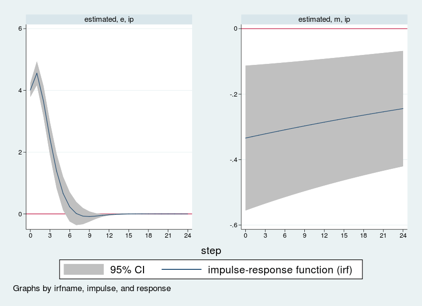
Each panel shows the response of industrial production to one shock. Because our data are measured in growth rates, the vertical axis is also measured in growth rates. Hence, a value of “4” in the left-hand panel means that after a one standard-deviation shock, industrial production grows four percentage points faster than it otherwise would. The horizontal axis is time; because we used monthly data, it is time in months, and 12 steps represents 1 year.
The left-hand panel shows the response of industrial production to a rise in e, the latent factor affecting production. Industrial production rises, peaking one period after the shock before settling back down to long-run equilibrium. The effect of the shock wears off quickly; industrial production returns to long-run equilibrium within 12 periods (1 year of monthly observations).
The right-hand panel shows the response of industrial production to a rise in m, which has a natural interpretation as an unexpected hike in interest rates. The size of a shock is one standard deviation, which from the dsge estimates table above is an unexpected rise in interest rates of about 0.546, or about one-half of one percentage point. In response, we see in the graph that industrial production growth falls by about one-third of one percentage point and remains low for over 24 periods. All variables in a DSGE model are stationary, so in the long run, the effect of a shock dies off, and the variables return to their long-run mean of zero.
Explore systematic policy: A change in regime
Next, we contemplate a shift in policy regime. Suppose the policymaker receives instructions to smooth out fluctuations in industrial production resulting from shocks to e. In terms of the model, this directive would be represented by a regime shift from the relatively low response coefficient beta seen in the data to a higher response coefficient.
dsge with the from() and solve options allows you to trace out an impulse response from any arbitrary parameter set. We will take advantage of this feature now. First, we store the estimated parameter vector in a Stata matrix:
. matrix b2 = e(b)
Next, we replace the coefficient beta with a larger response coefficient. For illustrative purposes, I use a response coefficient of 0.8 instead of 0.02. The old and new parameter vectors are
. matrix b2[1,2] = 0.8

. matlist e(b)

             | /struct~l                                             | /
             |     alpha       beta        rho     theta1     theta2 |   sd(e.m)
-------------+-------------------------------------------------------+-----------
          y1 | -.6287781   .0239873   .9870175    1.13085  -.3731307 |  .5464261

             | /
             |   sd(e.e)
-------------+-----------
          y1 |  4.079367

. matlist b2

             | /struct~l                                             | /
             |     alpha       beta        rho     theta1     theta2 |   sd(e.m)
-------------+-------------------------------------------------------+-----------
          y1 | -.6287781         .8   .9870175    1.13085  -.3731307 |  .5464261

             | /
             |   sd(e.e)
-------------+-----------
          y1 |  4.079367
As expected, they are identical except for the beta entry. Next, we rerun dsge at the new parameter vector with from() and solve.
. dsge (ip = {alpha}*E(F.r) + e)
>         (r = {beta}*ip + m )
>         (F.m = {rho}*m, state)
>         (F.e = {theta1}*e + {theta2}*Le, state)
>         (F.Le = e, state noshock)
>         , from(b2) solve

DSGE model

Sample: 1954m7 - 2006m12                        Number of obs     =        630
Log likelihood = -15344.268
------------------------------------------------------------------------------
             |                 OIM
             |      Coef.   Std. Err.      z    P>|z|     [95% Conf. Interval]
-------------+----------------------------------------------------------------
/structural  |
       alpha |  -.6287781          .        .       .            .           .
        beta |         .8          .        .       .            .           .
         rho |   .9870175          .        .       .            .           .
      theta1 |    1.13085          .        .       .            .           .
      theta2 |  -.3731307          .        .       .            .           .
-------------+----------------------------------------------------------------
      sd(e.m)|   .5464261          .                             .           .
      sd(e.e)|   4.079367          .                             .           .
------------------------------------------------------------------------------
Note: Model solved at specified parameters.
We use these new parameter values to create a new set of IRFs that we call counterfactual.
. irf create counterfactual, step(24)
(file dta/dsge_irf.irf updated)
Finally, we plot the responses under the estimated and counterfactual parameter vectors with irf ograph:
. irf ograph (estimated e ip irf) (counterfactual e ip irf),
> xlabel(0(3)24) yline(0)
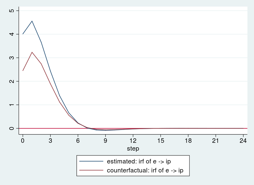
The more aggressive policy has dampened the response of industrial production to the e shock. The policymaker could experiment with other values of beta until he or she found a value that dampened the response of industrial production by the desired amount.
Appendix
Data
I used data on the growth rate of industrial production and on the Federal funds interest rate. Both of these series are available monthly at the St. Louis Federal Reserve database, FRED. The Stata command import fred imports data from FRED. The codes are INDPRO for industrial production and FEDFUNDS for the Federal funds rate.
I generate the variable ip as the annualized quarterly growth rate of industrial production and use a sample from 1954 to 2006.
. import fred INDPRO FEDFUNDS
. generate datem = mofd(daten)
. tsset datem, monthly
. generate ip = 400*ln(INDPRO / L3.INDPRO)
. label variable ip "Growth rate of industrial production"
. rename FEDFUNDS r
. label variable r "Federal funds rate"
. keep if yofd(daten) <= 2006
Specifying state equations with long lags
See also [DSGE] intro 4c.
Notice that state variables are written in a state-space form in terms of their one-period-ahead value. For an AR(1) process, this is easy. The equation
\begin{align*}
m_{t+1} &= \rho m_t + v_{t+1}
\end{align*}
becomes the following in Stata:
. dsge ... (F.m = {rho}*m, state) ...
But for an AR(2) process, the law of motion for the state variable is
\begin{align*}
e_{t+1} &= \theta_{1} e_t + \theta_{2} e_{t-1} + u_{t+1}
\end{align*}
which we split into two equations:
\begin{align*}
\begin{pmatrix} e_{t+1} \\ e_t \end{pmatrix}
=
\begin{pmatrix}
\theta_{1} & \theta_{2} \\
1 & 0 \\
\end{pmatrix}
\begin{pmatrix}
e_t \\ e_{t-1}
\end{pmatrix}
+
\begin{pmatrix}
u_t \\ 0
\end{pmatrix}
\end{align*}
These two equations become, in Stata,
. dsge ... (F.e = {theta1}*e + {theta2}*Le, state) (F.Le = e, state noshock) ...
where the noshock option in the last equation specifies that it is exact.
See also [TS] sspace example 5, where a similar trick is used.