Calculating power using Monte Carlo simulations, part 3: Linear and logistic regression
In my last two posts, I showed you how to calculate power for a t test using Monte Carlo simulations and how to integrate your simulations into Stata’s power command. In today’s post, I’m going to show you how to do these tasks for linear and logistic regression models. The strategy and overall structure of the programs for linear and logistic regression are similar to the t test examples. The parts that will change are the simulation of the data and the models used to test the null hypothesis.
Choosing realistic regression parameters is challenging when simulating regression models. Sometimes, pilot data or historical data can provide clues, but often we must consider a range of parameter values that we believe are realistic. I am going to deal with this challenge by working examples that are based on the data from the National Health and Nutrition Examination Survey (NHANES). You can download a version of these data by typing webuse nhanes2.
Linear regression example
Let’s imagine that you are planning a study of systolic blood pressure (SBP) and you believe that there is an interaction between age and sex. The NHANES dataset includes the variables bpsystol (SBP), age, and sex. Below, I have fit a linear regression model that includes an age-by-sex interaction term, and the p-values for all the parameter estimates equal 0.000. This is not surprising, because the dataset includes 10,351 observations. p-values become smaller as sample sizes become larger when everything else is held constant.
. webuse nhanes2

. regress bpsystol c.age##ib1.sex

      Source |       SS           df       MS      Number of obs   =    10,351
-------------+----------------------------------   F(3, 10347)     =   1180.87
       Model |     1437147         3      479049   Prob > F        =    0.0000
    Residual |  4197523.03    10,347  405.675367   R-squared       =    0.2551
-------------+----------------------------------   Adj R-squared   =    0.2548
       Total |  5634670.03    10,350  544.412563   Root MSE        =    20.141

------------------------------------------------------------------------------
    bpsystol |      Coef.   Std. Err.      t    P>|t|     [95% Conf. Interval]
-------------+----------------------------------------------------------------
         age |     .47062   .0167357    28.12   0.000     .4378147    .5034252
             |
         sex |
     Female  |  -20.45813   1.165263   -17.56   0.000    -22.74227   -18.17398
             |
   sex#c.age |
     Female  |   .3457346   .0230373    15.01   0.000      .300577    .3908923
             |
       _cons |   110.5691   .8440692   131.00   0.000     108.9146    112.2236
------------------------------------------------------------------------------
Perhaps you don’t have the resources to collect a sample of 10,351 participants for your study, but you would like to have 80% power to detect an interaction parameter of 0.35. How large does your sample need to be?
Let’s start by creating a single pseudo-random dataset based on the parameter estimates from the NHANES model. We begin the code block below by clearing Stata’s memory. Next, we set the random seed to 15 so that we can reproduce our results and set the number of observations to 100.
clear
set seed 15
set obs 100
generate age = runiformint(18,65)
generate female = rbinomial(1,0.5)
generate interact = age*female
generate e = rnormal(0,20)
generate sbp = 110 + 0.5*age + (-20)*female + 0.35*interact  + e
The fourth line of the code block generates a variable named age, which includes integers drawn from a uniform distribution on the interval [18,65].
The fifth line generates an indicator variable named female using a Bernoulli distribution with probability equal to 0.5. Recall that a binomial distribution with one trial is equivalent to a Bernoulli distribution.
The sixth line generates a variable for the interaction of age and female.
The seventh line generates a variable, e, that is the error term for the regression model. The errors are generated from a normal distribution with a mean of 0 and standard deviation of 20. The value of 20 is based on the root MSE estimated from the NHANES regression model.
The last line of the code block generates the variable sbp based on a linear combination of our simulated variables and the parameter estimates from the NHANES regression model.
Below are the results of a linear model fit to our simulated data using regress. The parameter estimates differ somewhat from our input parameters because I generated only one relatively small dataset. We could reduce this discrepancy by increasing our sample size, drawing many samples, or both.
. regress sbp age i.female c.age#i.female

      Source |       SS           df       MS      Number of obs   =       100
-------------+----------------------------------   F(3, 96)        =      7.15
       Model |  9060.32024         3  3020.10675   Prob > F        =    0.0002
    Residual |  40569.7504        96  422.601567   R-squared       =    0.1826
-------------+----------------------------------   Adj R-squared   =    0.1570
       Total |  49630.0707        99  501.313845   Root MSE        =    20.557

------------------------------------------------------------------------------
         sbp |      Coef.   Std. Err.      t    P>|t|     [95% Conf. Interval]
-------------+----------------------------------------------------------------
         age |   .7752417   .1883855     4.12   0.000     .4012994    1.149184
    1.female |   5.759113   15.09611     0.38   0.704    -24.20644    35.72466
             |
female#c.age |
          1  |  -.2690026   .3319144    -0.81   0.420    -.9278475    .3898423
             |
       _cons |   100.4409   8.381869    11.98   0.000     83.80306    117.0788
------------------------------------------------------------------------------
The p-value for the interaction term equals 0.420, which is not statistically significant at the 0.05 level. Obviously, we need a larger sample size.
We could use the p-value from the regression model to test the null hypothesis that the interaction term is zero. That would work in this example because we are testing only one parameter. But we would have to test multiple parameters simultaneously if our interaction included a categorical variable such as race. And there may be times when we wish to test multiple variables simultaneously.
Likelihood-ratio tests can test many kinds of hypotheses, including multiple parameters simultaneously. I’m going to show you how to use a likelihood-ratio test in this example because it will generalize to other hypotheses you may encounter in your research. You can read more about likelihood-ratio tests in the Stata Base Reference Manual if you are not familiar with them.
The code block below shows four of the five steps used to calculate a likelihood-ratio test. We will test the null hypothesis that the coefficient for the interaction term equals zero. The first line fits the “full” regression model that includes the interaction term. The second line stores the estimates of the full model in memory. The name “full” is arbitrary. We could have named the results of this model anything we like. The third line fits the “reduced” regression model that omits the interaction term. And the fourth line stores the results of the reduced model in memory.
regress sbp age i.female c.age#i.female
estimates store full
regress sbp age i.female
estimates store reduced
The fifth step uses lrtest to calculate a likelihood-ratio test of the full model versus the reduced model. The test yields a p-value of 0.4089, which is close to the Wald test reported in the regression output above. We cannot reject the null hypothesis that the interaction parameter is zero.
. lrtest full reduced

Likelihood-ratio test                                 LR chi2(1)  =      0.68
(Assumption: reduced nested in full)                  Prob > chi2 =    0.4089
You can type return list to see that the p-value is stored in the scalar r(p). And you can use r(p) to define reject the same way we did in our t test program.
. return list

scalars:
                  r(p) =  .4089399864598747
               r(chi2) =  .6818803412616035
                 r(df) =  1

. local reject = (r(p)<0.05)
Simulating the data and testing the null hypothesis for a regression model are a little more complicated than for a t test. But writing a program to automate this process is almost identical to the t test example. Let’s consider the code block below, which defines the program simregress.
capture program drop simregress
program simregress, rclass
    version 16
    // DEFINE THE INPUT PARAMETERS AND THEIR DEFAULT VALUES
    syntax, n(integer)          /// Sample size
          [ alpha(real 0.05)    /// Alpha level
            intercept(real 110) /// Intercept parameter
            age(real 0.5)       /// Age parameter
            female(real -20)    /// Female parameter
            interact(real 0.35) /// Interaction parameter
            esd(real 20) ]      //  Standard deviation of the error
    quietly {
        // GENERATE THE RANDOM DATA
        clear
        set obs `n'
        generate age = runiformint(18,65)
        generate female = rbinomial(1,0.5)
        generate interact = age*female
        generate e = rnormal(0,`esd')
        generate sbp = `intercept' + `age'*age + `female'*female + ///
           `interact'*interact  + e
        // TEST THE NULL HYPOTHESIS
        regress sbp age i.female c.age#i.female
        estimates store full
        regress sbp age i.female
        estimates store reduced
        lrtest full reduced
    }
    // RETURN RESULTS
    return scalar reject = (r(p)<`alpha')
end
The first three lines, which begin with capture program, program, and version, are basically the same as in our t test program.
The syntax section of the program is similar to that of the t test program, but the names of the input parameters are, obviously, different. I have included input parameters for the sample size, alpha level, and basic regression parameters. I have not included an input parameter for every possible parameter in the model, but you could if you like. For example, I have “hard coded” the range of the variable age as 18 to 65 in my program. But you could include an input parameter for the upper and lower bounds of age if you wish. I also find it helpful to include comments that describe the parameter names so that there is no ambiguity.
The next section of code is embedded in a “quietly” block. Commands like set obs, generate, and regress send output to the Results window and log file (if you have one open). Placing these commands in a quietly block suppresses that output.
We have already written the commands to create our random data and test the null hypothesis. So we can copy that code into the quietly block and replace any input parameters with their corresponding local macros defined by syntax. For example, I have changed set obs 100 to set obs `n’ so that the number of observations will be set by the input parameter specified with syntax. I have also given the input parameters the same names as the simulated variables in the model. So `age’*age is the product of the input parameter `age’ defined by syntax and the variable age generated by simulation.
The p-value from the likelihood-ratio test is stored in the scalar r(p), and our program returns the scalar reject exactly as it did in our t test program.
Below, I have used simulate to run simregress 100 times and summarized the variable reject. The results indicate that we would have 16% power to detect an interaction parameter of 0.35 given a sample of 100 participants and the other assumptions about the model.
. simulate reject=r(reject), reps(100):
>         simregress, n(100) age(0.5) female(20) interact(0.35)
>            esd(20) alpha(0.05)

      command:  simregress, n(100) age(0.5) female(20) interact(0.35)
> esd(20) alpha(0.05)
       reject:  r(reject)

Simulations (100)
----+--- 1 ---+--- 2 ---+--- 3 ---+--- 4 ---+--- 5
..................................................    50
..................................................   100

. summarize reject

    Variable |        Obs        Mean    Std. Dev.       Min        Max
-------------+---------------------------------------------------------
      reject |        100         .16    .3684529          0          1
Next, let’s write a program called power_cmd_simregress so that we can integrate simregress into Stata’s power command. The structure of power_cmd_simregress is the same as power_cmd_ttest in my last post. First, we define the syntax and input parameters and specify their default values. Then, we run the simulation and summarize the variable reject. And finally, we return the results.
capture program drop power_cmd_simregress
program power_cmd_simregress, rclass
    version 16
    // DEFINE THE INPUT PARAMETERS AND THEIR DEFAULT VALUES
    syntax, n(integer)          /// Sample size
          [ alpha(real 0.05)    /// Alpha level
            intercept(real 110) /// Intercept parameter
            age(real 0.5)       /// Age parameter
            female(real -20)    /// Female parameter
            interact(real 0.35) /// Interaction parameter
            esd(real 20)        /// Standard deviation of the error
            reps(integer 100)]  //   Number of repetitions

    // GENERATE THE RANDOM DATA AND TEST THE NULL HYPOTHESIS
    quietly {
        simulate reject=r(reject), reps(`reps'):               ///
             simregress, n(`n') age(`age') female(`female')    ///
                         interact(`interact') esd(`esd') alpha(`alpha')
        summarize reject
    }
    // RETURN RESULTS
    return scalar power = r(mean)
    return scalar N = `n'
    return scalar alpha = `alpha'
    return scalar intercept = `intercept'
    return scalar age = `age'
    return scalar female = `female'
    return scalar interact = `interact'
    return scalar esd = `esd'
end
Let’s also write a program called power_cmd_simregress_init. Recall from my last post that this program will allow us to run power simregress for a range of input parameter values, including the parameters listed in double quotes.
capture program drop power_cmd_simregress_init
program power_cmd_simregress_init, sclass
    sreturn local pss_colnames "intercept age female interact esd"
    sreturn local pss_numopts  "intercept age female interact esd"
end
Now, we’re ready to use power simregress! The output below shows the simulated power when the interaction parameter equals 0.2 to 0.4 in increments of 0.05 for samples of size 400, 500, 600, and 700.
. power simregress, n(400(100)700) intercept(110)                 ///
>                   age(0.5) female(-20) interact(0.2(0.05)0.4)   ///
>                   reps(1000) table graph(xdimension(interact)   ///
>                   legend(rows(1)))

Estimated power
Two-sided test

  +--------------------------------------------------------------------+
  |   alpha   power       N intercept     age  female interact     esd |
  |--------------------------------------------------------------------|
  |     .05    .267     400       110      .5     -20       .2      20 |
  |     .05    .398     400       110      .5     -20      .25      20 |
  |     .05    .547     400       110      .5     -20       .3      20 |
  |     .05    .677     400       110      .5     -20      .35      20 |
  |     .05    .792     400       110      .5     -20       .4      20 |
  |     .05     .33     500       110      .5     -20       .2      20 |
  |     .05     .46     500       110      .5     -20      .25      20 |
  |     .05    .646     500       110      .5     -20       .3      20 |
  |     .05    .763     500       110      .5     -20      .35      20 |
  |     .05    .854     500       110      .5     -20       .4      20 |
  |     .05    .384     600       110      .5     -20       .2      20 |
  |     .05    .563     600       110      .5     -20      .25      20 |
  |     .05    .702     600       110      .5     -20       .3      20 |
  |     .05    .841     600       110      .5     -20      .35      20 |
  |     .05    .928     600       110      .5     -20       .4      20 |
  |     .05    .444     700       110      .5     -20       .2      20 |
  |     .05    .641     700       110      .5     -20      .25      20 |
  |     .05    .793     700       110      .5     -20       .3      20 |
  |     .05    .904     700       110      .5     -20      .35      20 |
  |     .05    .958     700       110      .5     -20       .4      20 |
  +--------------------------------------------------------------------+
Figure 1 displays the results graphically.
Figure 1: Estimated power for the interaction term in a regression model
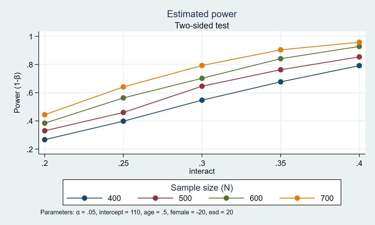
The table and the graph show us that there are several combinations of parameters that would result in 80% power. A sample of 700 participants would give us roughly 80% power to detect an interaction parameter of 0.30. A sample of 600 participants would give us roughly 80% power to detect an interaction parameter of 0.33. A sample of 500 participants would give us roughly 80% power to detect an interaction parameter of approximately 0.37. And a sample of 400 participants would give us roughly 80% power to detect an interaction parameter of 0.40. Our final choice of sample size is then based on the size of the interaction parameter that we would like to detect.
This example focused on the interaction term in a regression model with two covariates. But you could modify this example to simulate power for almost any kind of regression model you can imagine. I would suggest the following steps when planning your simulation:
- Write down the regression model of interest, including all parameters.
- Specify the details of the covariates, such as the range of age or the proportion of females.
- Locate or think about reasonable values for the parameters in your model.
- Simulate a single dataset assuming the alternative hypothesis, and fit the model.
- Write a program to create the datasets, fit the models, and use simulate to test the program.
- Write a program called power_cmd_mymethod, which allows you to run your simulations with power.
- Write a program called power_cmd_mymethod_init so that you can use numlists for all parameters.
Let’s try this approach for a logistic regression model.
Logistic regression example
In this example, let’s imagine that you are planning a study of hypertension (highbp). Hypertension is binary, so we will use logistic regression to fit the model and use odds ratios for the effect size.
Step 1: Write down the model
The first step toward simulating power is to write down the model.
\[
{\rm logit}({\bf highbp}) = \beta_0 + \beta_1({\bf age}) + \beta_2({\bf sex}) + \beta_3({\bf age}\times {\bf sex})
\]
We will need to create variables for highbp, age, sex, and the interaction term age\(\times \)sex. We will also need to specify reasonable parameter values for \(\beta_0\), \(\beta_1\), \(\beta_2\), and \(\beta_3\).
Step 2: Specify details of the covariates
Next, we need to think about the covariates in our model. What values of age are reasonable for our study? Are we interested in older adults? Younger adults? Let’s assume that we’re interested in adults between the ages of 18 and 65. Is the distribution of age likely to be uniform over the interval [18,65], or do we expect a hump-shaped distribution around the middle of the age range? We also need to think about the proportion of males and females in our study. Are we likely to sample 50% males and 50% females? These are the kinds of questions that we need to ask ourselves when planning our power calculations.
Let’s assume that we are interested in adults between the ages of 18 and 65 and we believe that age is uniformly distributed. Let’s also assume that the sample will be 50% female. The interaction term age\(\times \)sex is easy to calculate once we create variables for age and sex.
Step 3: Specify reasonable values for the parameters
Next we need to think about reasonable values for the parameters in our model. We could choose parameter values based on a review of the literature, results from a pilot study, or publicly available data.
I have chosen to use the NHANES data again because it includes the variables hypertension (highbp), age, and sex.
. webuse nhanes2

. logistic highbp c.age##ib1.sex

Logistic regression                             Number of obs     =     10,351
                                                LR chi2(3)        =    1675.19
                                                Prob > chi2       =     0.0000
Log likelihood = -6213.1696                     Pseudo R2         =     0.1188

------------------------------------------------------------------------------
      highbp | Odds Ratio   Std. Err.      z    P>|z|     [95% Conf. Interval]
-------------+----------------------------------------------------------------
         age |   1.035184   .0018459    19.39   0.000     1.031572    1.038808
             |
         sex |
     Female  |   .1556985   .0224504   -12.90   0.000     .1173677    .2065477
             |
   sex#c.age |
     Female  |   1.028811    .002794    10.46   0.000      1.02335    1.034302
             |
       _cons |   .1690035   .0153794   -19.54   0.000     .1413957    .2020018
------------------------------------------------------------------------------
Note: _cons estimates baseline odds.
The output includes estimates of the odds ratio for each of the variables in our model. Odds ratios are exponentiated parameter estimates (that is, \(\hat{{\rm OR}_i} = e^{\hat{\beta_i}}\)), so we could specify the natural logarithms of the odds ratios, \(\beta_i = {\rm ln}({\rm OR}_i)\), as parameters in our power simulations.
For example, the estimate of the odds ratio for age in the output above is 1.04, so we can specify \(\beta_1 = {\rm ln}(\hat{{\rm OR}_{\bf age}}) = {\rm ln}(1.04) \).
We can also specify \(\beta_0 = {\rm ln}(\hat{{\rm OR}_{\bf cons}}) = {\rm ln}(0.17) \), \(\beta_2 = {\rm ln}(\hat{{\rm OR}_{\bf sex}}) = {\rm ln}(0.16) \), and \(\beta_3 = {\rm ln}(\hat{{\rm OR}_{{\bf age}\times {\bf sex}}}) = {\rm ln}(1.03) \).
Step 4: Simulate a dataset assuming the alternative hypothesis, and fit the model
Next, we create a simulated dataset based on our assumptions about the model under the alternative hypothesis. The code block below is almost identical to the code we used to create the data for our linear regression model, but there are two important differences. First, we use generate xb to create a linear combination of the parameters and the simulated variables. The parameters are expressed as the natural logarithms of the odds ratios estimated with the NHANES data. Second, we use rlogistic(m,s) to create the binary dependent variable highbp from the variable xb.
clear
set seed 123456
set obs 100
generate age = runiformint(18,65)
generate female = rbinomial(1,0.5)
generate interact = age*female
generate xb = (ln(0.17) + ln(1.04)*age + ln(0.15)*female + ln(1.03)*interact)
generate highbp = rlogistic(xb,1) > 0
We can then fit a logistic regression model to our simulated data.
. logistic highbp age i.female c.age#i.female

Logistic regression                             Number of obs     =        100
                                                LR chi2(3)        =      14.95
                                                Prob > chi2       =     0.0019
Log likelihood = -61.817323                     Pseudo R2         =     0.1079

------------------------------------------------------------------------------
      highbp | Odds Ratio   Std. Err.      z    P>|z|     [95% Conf. Interval]
-------------+----------------------------------------------------------------
         age |   1.055245   .0250921     2.26   0.024     1.007194    1.105589
    1.female |   .2365046   .3730999    -0.91   0.361     .0107404    5.207868
             |
female#c.age |
          1  |   1.015651   .0365417     0.43   0.666     .9464976    1.089857
             |
       _cons |   .1578931    .151025    -1.93   0.054     .0242207    1.029293
------------------------------------------------------------------------------
Note: _cons estimates baseline odds.
Step 5: Write a program to create the datasets, fit the models, and use simulate to test the program
Next, let’s write a program that creates datasets under the alternative hypothesis, fits logistic regression models, tests the null hypothesis, and uses simulate to run many iterations of the program.
The code block below contains the syntax for a program named simlogit. The default parameter values in the syntax command are the odds ratios that we estimated using the NHANES data. And we use lrtest to test the null hypothesis that the odds ratio for the age\(\times \)sex interaction equals 1.
capture program drop simlogit
program simlogit, rclass
    version 16
    // DEFINE THE INPUT PARAMETERS AND THEIR DEFAULT VALUES
    syntax, n(integer)              /// Sample size
          [ alpha(real 0.05)        /// Alpha level
            intercept(real 0.17)    /// Intercept odds ratio
            age(real 1.04)          /// Age odds ratio
            female(real 0.15)       /// Female odds ratio
            interact(real 1.03) ]   //  Interaction odds ratio
    // GENERATE THE RANDOM DATA AND TEST THE NULL HYPOTHESIS
    quietly {
        drop _all
        set obs `n'
        generate age = runiformint(18,65)
        generate female = rbinomial(1,0.5)
        generate interact = age*female
        generate xb = (ln(`intercept') + ln(`age')*age + ln(`female')*female + ln(`interact')*interact)
        generate highbp = rlogistic(xb,1) > 0

        logistic highbp age i.female c.age#i.female
        estimates store full
        logistic highbp age i.female
        estimates store reduced
        lrtest full reduced
    }
    // RETURN RESULTS
    return scalar reject = (r(p)<`alpha')
end
We then use simulate to run simlogit 100 times using the default parameter values.
. simulate reject=r(reject), reps(100):   ///
>         simlogit, n(500) intercept(0.17) age(1.04) female(.15) interact(1.03) alpha(0.05)

      command:  simlogit, n(500) intercept(0.17) age(1.04) female(.15)
> interact(1.03) alpha(0.05)
       reject:  r(reject)

Simulations (100)
----+--- 1 ---+--- 2 ---+--- 3 ---+--- 4 ---+--- 5
..................................................    50
..................................................   100
simulate saved the results of the hypothesis tests to a variable named reject. The mean of reject is our estimate of the power to detect an odds ratio of 1.03 for the age\(\times \)sex interaction term assuming a sample size of 500 people.
. summarize reject

    Variable |        Obs        Mean    Std. Dev.       Min        Max
-------------+---------------------------------------------------------
      reject |        100         .53    .5016136          0          1
Step 6: Write a program called power_cmd_simlogit
We could stop with our quick simulation if we were interested only in a specific set of assumptions. But it’s easy to write an additional program called power_cmd_simlogit which will allow us to use Stata’s power command to create tables and graphs for a range of sample sizes.
capture program drop power_cmd_simlogit
program power_cmd_simlogit, rclass
    version 16
    // DEFINE THE INPUT PARAMETERS AND THEIR DEFAULT VALUES
    syntax, n(integer)              /// Sample size
          [ alpha(real 0.05)        /// Alpha level
            intercept(real 0.17)    /// Intercept odds ratio
            age(real 1.04)          /// Age odds ratio
            female(real 0.15)       /// Female odds ratio
            interact(real 1.03)     ///  Interaction odds ratio
            reps(integer 100) ]     //   Number of repetitions
    // GENERATE THE RANDOM DATA AND TEST THE NULL HYPOTHESIS
    quietly {
        simulate reject=r(reject), reps(`reps'):                      ///
                 simlogit, n(`n') intercept(`intercept') age(`age')   ///
                 female(`female') interact(`interact') alpha(`alpha')
        summarize reject
        local power = r(mean)
    }
    // RETURN RESULTS
    return scalar power = r(mean)
    return scalar N = `n'
    return scalar alpha = `alpha'
    return scalar intercept = `intercept'
    return scalar age = `age'
    return scalar female = `female'
    return scalar interact = `interact'
end
Step 7: Write a program called power_cmd_simlogit_init
It’s also easy to write a program called power_cmd_simlogit_init which will allow us to simulate power for a range of values for the parameters in our model.
capture program drop power_cmd_simlogit_init
program power_cmd_simlogit_init, sclass
    sreturn local pss_colnames "intercept age female interact"
    sreturn local pss_numopts  "intercept age female interact"
end
Using power simlogit
Now, we can use power simlogit to simulate power for a variety of assumptions. The example below simulates power for a range of sample sizes and effect sizes. Sample sizes range from 400 to 1000 people in increments of 200. And the odds ratios for the age\(\times \)sex interaction term range from 1.02 to 1.05 in increments of 0.01.
. power simlogit, n(400(200)1000) intercept(0.17) age(1.04) female(.15) interact(1.02(0.01)1.05)  ///
>                 reps(1000) table graph(xdimension(interact) legend(rows(1)))

Estimated power
Two-sided test

  +------------------------------------------------------------+
  |   alpha   power       N intercept     age  female interact |
  |------------------------------------------------------------|
  |     .05    .197     400       .17    1.04     .15     1.02 |
  |     .05    .423     400       .17    1.04     .15     1.03 |
  |     .05    .645     400       .17    1.04     .15     1.04 |
  |     .05    .797     400       .17    1.04     .15     1.05 |
  |     .05    .275     600       .17    1.04     .15     1.02 |
  |     .05    .602     600       .17    1.04     .15     1.03 |
  |     .05    .838     600       .17    1.04     .15     1.04 |
  |     .05    .927     600       .17    1.04     .15     1.05 |
  |     .05    .357     800       .17    1.04     .15     1.02 |
  |     .05    .675     800       .17    1.04     .15     1.03 |
  |     .05    .899     800       .17    1.04     .15     1.04 |
  |     .05    .987     800       .17    1.04     .15     1.05 |
  |     .05     .46   1,000       .17    1.04     .15     1.02 |
  |     .05    .791   1,000       .17    1.04     .15     1.03 |
  |     .05    .956   1,000       .17    1.04     .15     1.04 |
  |     .05    .993   1,000       .17    1.04     .15     1.05 |
  +------------------------------------------------------------+
Figure 2: Estimated power for the interaction term in a logistic regression model
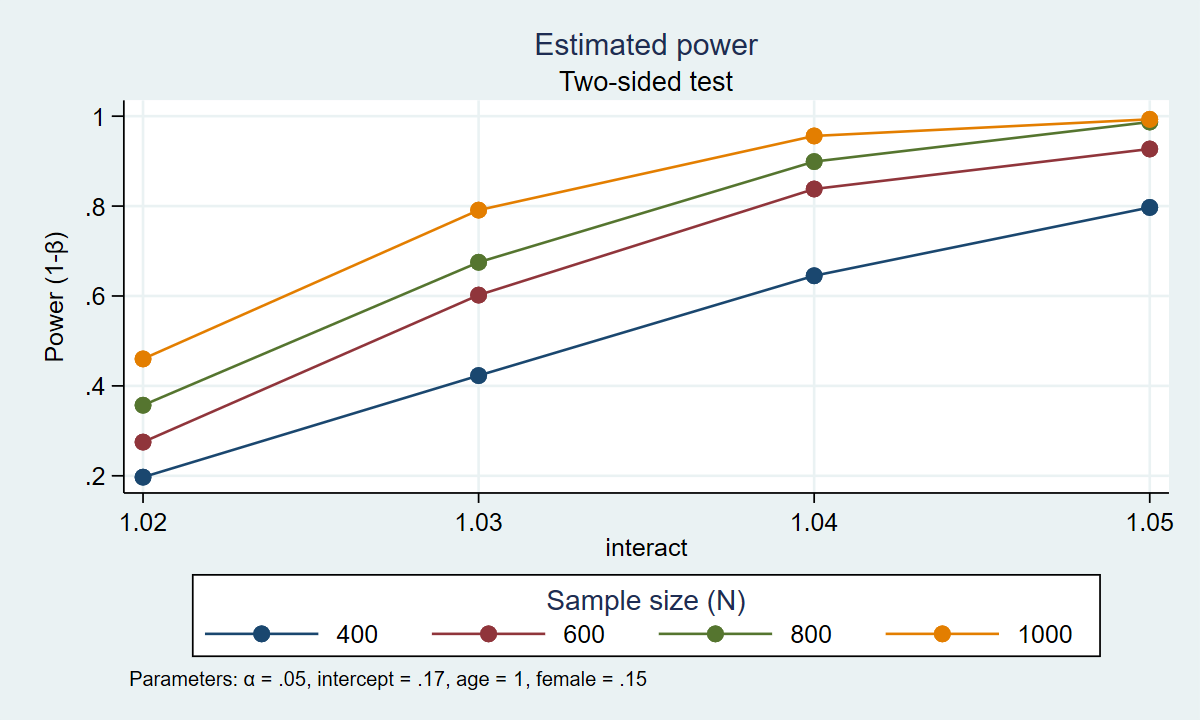
The table and graph above indicate that 80% power is achieved with four combinations of sample size and effect size. Given our assumptions, we estimate that we will have at least 80% power to detect an odds ratio of 1.04 for sample sizes of 600, 800, and 1000. And we estimate that we will have 80% power to detect an odds ratio of 1.05 with a sample size of 400 people.
In this blog post, I showed you how to simulate statistical power for the interaction term in both linear and logistic regression models. You may be interested in simulating power for variations of these models, and you can modify the examples above for your own purposes. In my next post, I will show you how to simulate power for multilevel and longitudinal models.