Calculating power using Monte Carlo simulations, part 4: Multilevel/longitudinal models
In my last three posts, I showed you how to calculate power for a t test using Monte Carlo simulations, how to integrate your simulations into Stata’s power command, and how to do this for linear and logistic regression models. In today’s post, I’m going to show you how to estimate power for multilevel/longitudinal models using simulations. You may want to review my earlier post titled “How to simulate multilevel/longitudinal data” before you read this post.
Our goal is to write a program that will calculate power for different values of the model parameters. For example, figure 1 displays power for different numbers of observations at level 1 and 2 in a longitudinal model.
Figure 1: Estimated power for a multilevel/longitudinal model
In my last post, I suggested the following steps for writing such a program, so let’s follow these steps again for a multilevel/longitudinal model.
- Write down the regression model of interest, including all parameters.
- Specify the details of the covariates, such as the range of age or the proportion of females.
- Locate or think about reasonable values for the parameters in your model.
- Simulate a single dataset assuming the alternative hypothesis, and fit the model.
- Write a program to create the datasets, fit the models, and use simulate to test the program.
- Write a program called power_cmd_mymethod, which allows you to run your simulations with power.
- Write a program called power_cmd_mymethod_init so that you can use numlists for all parameters.
In this example, let’s imagine that you are planning a longitudinal study of childrens’ weight and you are interested in the interaction of age and sex.
Step 1: Write down the model
The first step toward simulating power is to write down the model.
\[
{\bf weight}_{it} = \beta_0 + \beta_1({\bf age}_{it}) + \beta_2({\bf female}_i) + \beta_3({\bf age}_{it}\times {\bf female}_i) + u_{0i} + u_{1i}({\bf age}) + e_{it}
\]
Here i indexes children, t indexes time (age), and we assume that \(u_{0i} \sim N(0,\tau_0)\), \(u_{1i} \sim N(0,\tau_1)\), \(e_{it} \sim N(0,\sigma)\), and \({\rm cov}(\tau_0,\tau_1)=0\).
We will need to create variables for weight, age, female, and the interaction term age\(\times \)female. We will also need to specify reasonable parameter values for \(\beta_0\), \(\beta_1\), \(\beta_2\), \(\beta_3\), \(\tau_0\), \(\tau_1\), and \(\sigma\).
Step 2: Specify the details of the covariates
Next, we need to think about the covariates in our model. This is a longitudinal study, so we need to specify the starting age, the length of time between measurements, and the total number of measurements. We also need to consider the proportion of males and females in our study. Are we likely to sample 50% females and 50% males?
Let’s assume that we will measure the childrens’ weight every 6 months for 2 years beginning at age 12. And let’s also assume that the sample will be 50% female. The interaction term age\(\times \)female is easy to calculate once we create variables for age and female.
Step 3: Locate or think about reasonable values for the parameters in your model
Next, we need to think about reasonable values for the parameters in our model. We could choose parameter values based on a review of the literature, results from a pilot study, or from publicly available data.
I have chosen to use data from a study of the weight of Asian children. You can download and describe this dataset by typing
. use http://www.stata-press.com/data/r16/childweight.dta, clear
(Weight data on Asian children)

. describe

Contains data from http://www.stata-press.com/data/r16/childweight.dta
  obs:           198                          Weight data on Asian children
 vars:             5                          23 May 2016 15:12
 size:         3,168                          (_dta has notes)
--------------------------------------------------------------------------------
              storage   display    value
variable name   type    format     label      variable label
--------------------------------------------------------------------------------
id              int     %8.0g                 child identifier
age             float   %8.0g                 age in years
weight          float   %8.0g                 weight in Kg
brthwt          int     %8.0g                 Birth weight in g
girl            float   %9.0g      bg         gender
--------------------------------------------------------------------------------
Sorted by: id  age
This dataset includes variables for age measured in years (age), weight measured in kilograms (weight), and gender (girl). We can verify that these are longitudinal data by listing some of the observations.
. list in 1/5

     +---------------------------------------+
     | id       age   weight   brthwt   girl |
     |---------------------------------------|
  1. | 45   .136893    5.171     4140    boy |
  2. | 45   .657084    10.86     4140    boy |
  3. | 45   1.21834    13.15     4140    boy |
  4. | 45   1.42916     13.2     4140    boy |
  5. | 45   2.27242    15.88     4140    boy |
     +---------------------------------------+
Child 45 is a boy whose weight was recorded five times over two years. Notice that age is not stored as absolute age. It is stored as decimals representing the number of years since an unknown point in time. This isn’t a problem because we are interested in the change of weight over time. We can fit our model to this dataset to estimate the parameters.
. mixed weight c.age##i.girl || id: age, stddev

Performing EM optimization:

Performing gradient-based optimization:

Iteration 0:   log likelihood = -339.79909
Iteration 1:   log likelihood = -339.41232
Iteration 2:   log likelihood = -339.41033
Iteration 3:   log likelihood = -339.41032

Computing standard errors:

Mixed-effects ML regression                     Number of obs     =        198
Group variable: id                              Number of groups  =         68

                                                Obs per group:
                                                              min =          1
                                                              avg =        2.9
                                                              max =          5

                                                Wald chi2(3)      =     680.51
Log likelihood = -339.41032                     Prob > chi2       =     0.0000

------------------------------------------------------------------------------
      weight |      Coef.   Std. Err.      z    P>|z|     [95% Conf. Interval]
-------------+----------------------------------------------------------------
         age |   3.588488   .1892333    18.96   0.000     3.217598    3.959379
             |
        girl |
       girl  |   -.468204   .2954284    -1.58   0.113    -1.047233     .110825
             |
  girl#c.age |
       girl  |  -.2397793    .267607    -0.90   0.370    -.7642793    .2847208
             |
       _cons |   5.351429   .2076606    25.77   0.000     4.944421    5.758436
------------------------------------------------------------------------------

------------------------------------------------------------------------------
  Random-effects Parameters  |   Estimate   Std. Err.     [95% Conf. Interval]
-----------------------------+------------------------------------------------
id: Independent              |
                     sd(age) |   .5662947   .1219764      .3712777    .8637461
                   sd(_cons) |   .2384136   .4034962      .0086445    6.575403
-----------------------------+------------------------------------------------
                sd(Residual) |   1.165676   .0762599      1.025395    1.325148
------------------------------------------------------------------------------
LR test vs. linear model: chi2(2) = 20.38                 Prob > chi2 = 0.0000

Note: LR test is conservative and provided only for reference.
We can use the parameter estimates from this model to help us choose the parameters for our simulation. For example, we could begin our simulation by setting the simulation parameters equal to the parameter estimates above: \(\beta_0=5.35\), \(\beta_1=3.59\), \(\beta_2=-0.47\), \(\beta_3=-0.24\), \(\tau_0=0.24\), \(\tau_1=0.57\), and \(\sigma=1.17\).
Step 4: Simulate a single dataset assuming the alternative hypothesis, and fit the model
Next, we create a simulated dataset based on our assumptions about the model under the alternative hypothesis. We will simulate 5 observations at 6-month increments for 200 children. You may wish to read my previous blog post titled “How to simulate multilevel/longitudinal data” if you have not done this before.
The code block below is similar to the code we used to create the data for our linear regression model, but there are two features that are unique to simulating multilevel data. First, we generate the child-level variables child and female as well as the random deviations u_0i and u_1i. Second, we use expand to make five copies of the observations for each child. Third, we use bysort child: to generate age within each child. Fourth, we generate the observation-level variable interaction and the observation-level error (e_ij). Finally, we generate the variable weight using a linear combination of parameter values and the other variables that we generated.
set seed 16
clear
set obs 200
generate child = _n
generate female = rbinomial(1,0.5)
generate u_0i = rnormal(0,0.25)
generate u_1i = rnormal(0,0.60)
expand 5
bysort child: generate age = (_n-1)*0.5
generate interaction = age*female
generate e_ij = rnormal(0,1.2)
generate weight = 5.35 + 3.6*age + (-0.5)*female + (-0.25)*interaction ///
    + u_0i + age*u_1i + e_ij
Let’s list the data for child 1 to check our work. The simulated data includes five observations for weight, age, and female. Our dataset also includes the random deviations that we would not observe in a real dataset.
. list child weight age female u_0i u_1i e_ij if child==1

      +------------------------------------------------------------------+
      | child     weight   age   female       u_0i       u_1i       e_ij |
      |------------------------------------------------------------------|
   1. |     1   6.957936     0        1   .0530039   .6878794   2.054933 |
   2. |     1   8.517486    .5        1   .0530039   .6878794   1.595542 |
   3. |     1   10.28054     1        1   .0530039   .6878794   1.339654 |
   4. |     1   11.48091   1.5        1   .0530039   .6878794   .5210837 |
   5. |     1   14.25277     2        1   .0530039   .6878794   1.274008 |
      +------------------------------------------------------------------+
We can then use mixed to fit a model to our simulated data.
. mixed weight age i.female c.age#i.female || child: age , stddev nolog noheader

------------------------------------------------------------------------------
      weight |      Coef.   Std. Err.      z    P>|z|     [95% Conf. Interval]
-------------+----------------------------------------------------------------
         age |   3.654038   .1029402    35.50   0.000     3.452279    3.855797
    1.female |  -.3765285   .1389315    -2.71   0.007    -.6488291   -.1042279
             |
female#c.age |
          1  |  -.4101041    .142071    -2.89   0.004    -.6885581   -.1316501
             |
       _cons |   5.309637   .1006654    52.75   0.000     5.112336    5.506937
------------------------------------------------------------------------------

------------------------------------------------------------------------------
  Random-effects Parameters  |   Estimate   Std. Err.     [95% Conf. Interval]
-----------------------------+------------------------------------------------
child: Independent           |
                     sd(age) |   .6628522   .0544682      .5642497    .7786855
                   sd(_cons) |   .3342406   .1071213       .178343    .6264151
-----------------------------+------------------------------------------------
                sd(Residual) |   1.190916   .0316823      1.130411    1.254659
------------------------------------------------------------------------------
LR test vs. linear model: chi2(2) = 157.47                Prob > chi2 = 0.0000

Note: LR test is conservative and provided only for reference.
We can then test the null hypothesis that the interaction term equals zero using a likelihood-ratio test. Recall from my last post that we can calculate a likelihood-ratio test by fitting the model with and without the intereaction term female#c.age and use lrtest to calculate the test statistic.
mixed weight age i.female c.age#i.female || child: age , stddev nolog noheader
estimates store full
mixed weight age i.female || child: age , stddev nolog noheader
estimates store reduced
lrtest full reduced
The p-value for our test is 0.0041, so we would reject the null hypothesis that the interaction term equals zero.
. lrtest full reduced

Likelihood-ratio test                                 LR chi2(1)  =      8.23
(Assumption: reduced nested in full)                  Prob > chi2 =    0.0041
In this example, both models converged. But sometimes models fail to converge for some of the datasets when we fit models to many simulated datasets. This is often because the process of simulating data can result in data that are incompatible with the model. But there may be other reasons, and you should consider them carefully if you observe many models that fail to converge.
Lack of model convergence can also cause our simulation to run far longer than necessary. By default, mixed will run 16,000 maximum-likelihood iterations before it stops. In the code block below, I have added options and lines to handle models that fail to converge. The option iter(200) in the mixed commands will stop them from running if a model fails to converge in the first 200 iterations. mixed will store a value of 1 to e(converged) if the model converges and 0 otherwise. The second line of the code block stores the value of e(converged) from the first model to a local macro named conv1. The fifth line of the code block stores the value of e(converged) from the second model to a local macro named conv2. The last line of the code block stores a value to the local macro reject. The value that is stored in reject is determined by the conditional function cond(). If both mixed models converged and `conv1’+`conv2’==2, then r(p)<`alpha’ will be evaluated. A value of 1 will be stored to reject if the likelihood-ratio p-value, r(p), is less than the alpha level specified in `alpha’ and 0 otherwise. If either of the mixed models fails to converge and `conv1’+`conv2′ does not equal 2, then a missing value will be stored to reject.
mixed weight age i.female c.age#i.female || child: age, iter(200)
local conv1 = e(converged)
estimates store full
mixed weight age i.female || child: age, iter(200)
local conv2 = e(converged)
estimates store reduced
lrtest full reduced
local reject = cond(`conv1'+`conv2'==2, r(p)<`alpha', .)
Step 5: Write a program to create the datasets, fit the models, and use simulate to test the program
Next, let’s write a program that creates datasets under the alternative hypothesis, fits mixed models, tests the null hypothesis of interest, and uses simulate to run many iterations of the program.
The code block below contains the syntax for a program named simmixed. The default parameter values in the syntax command are similar to the parameters that we estimated using the Asian children dataset. And we use lrtest to test the null hypothesis that the parameter for the age\(\times \)female interaction equals zero.
capture program drop simmixed
program simmixed, rclass
    version 16
    // PARSE INPUT
    syntax, n1(integer)             ///
            n(integer)              ///
          [ alpha(real 0.05)        ///
            intercept(real 5.35)    ///
            age(real 3.6)           ///
            female(real -0.5)       ///
            interact(real -0.25)    ///
            u0i(real 0.25)          ///
            u1i(real 0.60)          ///
            eij(real 1.2) ]

    // COMPUTE POWER
    quietly {
        drop _all
        set obs `n'
        generate child = _n
        generate female = rbinomial(1,0.5)
        generate u_0i = rnormal(0,`u0i')
        generate u_1i = rnormal(0,`u1i')
        expand `n1'
        bysort child: generate age = (_n-1)*0.5
        generate interaction = age*female
        generate e_ij = rnormal(0,`eij')
        generate weight = `intercept' + `age'*age + `female'*female + ///
           `interact'*interaction  + u_0i + age*u_1i + e_ij

        mixed weight age i.female c.age#i.female || child: age, iter(200)
        local conv1 = e(converged)
        estimates store full
        mixed weight age i.female || child: age, iter(200)
        local conv2 = e(converged)
        estimates store reduced
        lrtest full reduced
        local reject = cond(`conv1' + `conv2'==2, (r(p)<`alpha'), .)
    }
    // RETURN RESULTS
    return scalar reject = `reject'
    return scalar conv = `conv1'+`conv2'
end
We then use simulate to run simmixed 10 times using the default parameter values for 5 observations on each of 200 children.
. simulate reject=r(reject) converged=r(conv), reps(10) seed(12345):
>              simmixed, n1(5) n(200)

      command:  simmixed, n1(5) n(200)
       reject:  r(reject)
    converged:  r(conv)

Simulations (10)
----+--- 1 ---+--- 2 ---+--- 3 ---+--- 4 ---+--- 5
..........
simulate saved the results of the hypothesis tests to a variable named reject. The mean of reject is our estimate of the power to test the null hypothesis that the age\(\times \)sex interaction term equals zero, assuming that the weight of 200 children is measured 5 times.
. summarize reject

    Variable |        Obs        Mean    Std. Dev.       Min        Max
-------------+---------------------------------------------------------
      reject |         10          .3    .4830459          0          1
Step 6: Write a program called power_cmd_mymethod, which allows you to run your simulations with power
We could stop with our quick simulation if we were interested only in a specific set of assumptions. But it’s easy to write an additional program named power_cmd_simmixed that will allow us to use Stata’s power command to create tables and graphs for a range of sample sizes.
capture program drop power_cmd_simmixed
program power_cmd_simmixed, rclass
    version 16
    // PARSE INPUT
    syntax, n1(integer)             ///
            n(integer)              ///
          [ alpha(real 0.05)        ///
            intercept(real 5.35)    ///
            age(real 3.6)           ///
            female(real -0.5)       ///
            interact(real -0.25)    ///
            u0i(real 0.25)          ///
            u1i(real 0.60)          ///
            eij(real 1.2)           ///
            reps(integer 1000) ]

    // COMPUTE POWER
    quietly {
        simulate reject=r(reject), reps(`reps'):                            ///
        simmixed, n1(`n1') n(`n') alpha(`alpha') intercept(`intercept')     ///
                  age(`age') female(`female') interact(`interact')          ///
                  u0i(`u0i') u1i(`u1i') eij(`eij')
        summarize reject
    }

    // RETURN RESULTS
    return scalar power = r(mean)
    return scalar n1 = `n1'
    return scalar N = `n'
    return scalar alpha = `alpha'
    return scalar intercept = `intercept'
    return scalar age = `age'
    return scalar female = `female'
    return scalar interact = `interact'
    return scalar u0i = `u0i'
    return scalar u1i = `u1i'
    return scalar eij = `eij'
end
Step 7: Write a program called power_cmd_mymethod_init so that you can use numlists for all parameters
It’s also easy to write a program named power_cmd_simmixed_init that will allow us to simulate power for a range of values for the parameters in our model.
capture program drop power_cmd_simmixed_init
program power_cmd_simmixed_init, sclass
      version 16
      sreturn clear
      // ADD COLUMNS TO THE OUTPUT TABLE
      sreturn local pss_colnames "n1 intercept age female interact u0i u1i eij"
      // ALLOW NUMLISTS FOR ALL PARAMETERS
      sreturn local pss_numopts  "n1 intercept age female interact u0i u1i eij"
end
Using power simmixed
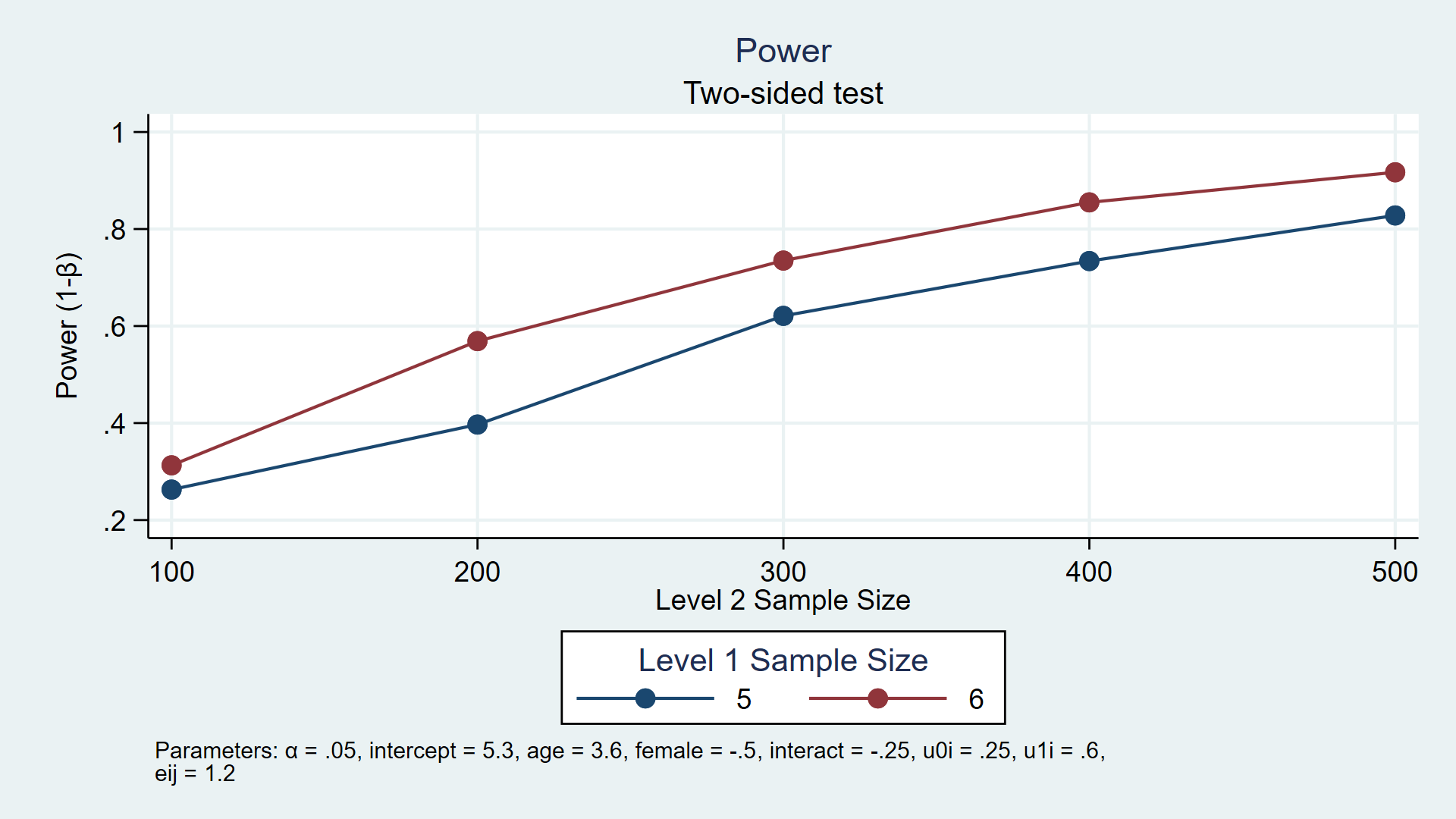
Now, we can use power simmixed to simulate power for a variety of assumptions. The example below simulates power for a range of sample sizes at both levels 1 and 2. Level 2 sample sizes range from 100 to 500 children in increments of 100. At level 1, we consider 5 and 6 observations per child.
. power simmixed, n1(5 6) n(100(100)500) reps(1000)
>               table(n1 N power)
>               graph(ydimension(power) xdimension(N) plotdimension(n1)
>               xtitle(Level 2 Sample Size) legend(title(Level 1 Sample Size)))
xxxxxxxxxxxxxxxxxxxxxxxxxxx
Estimated power
Two-sided test

  +-------------------------+
  |      n1       N   power |
  |-------------------------|
  |       5     100   .2629 |
  |       6     100    .313 |
  |       5     200    .397 |
  |       6     200    .569 |
  |       5     300    .621 |
  |       6     300    .735 |
  |       5     400    .734 |
  |       6     400    .855 |
  |       5     500    .828 |
  |       6     500    .917 |
  +-------------------------+
Figure 2: Estimated power for a multilevel/longitudinal model
The table and graph above indicate that 80% power is achieved with three combinations of sample sizes. Given our assumptions, we estimate that we will have at least 80% power to detect an interaction parameter of -0.25 with 400 children measured 6 times each and 500 children measured 5 or 6 times each.
Running our simulations with power gives us the flexibility to use power simmixed to estimate power for different values of any model parameter we wish. For example, we could consider different values of the interaction term along with different numbers of observations per child.
In this blog post, I showed you how to simulate statistical power for the interaction term in a multilevel regression model. You may be interested in simulating power for variations of these models, and you can modify this example for your own purposes. In my next post, I will show you how to simulate power for path coefficients in structural equation models.