Revealed preference: Stata for reproducible research
I care about reproducible research. Anyone who has ever been a research assistant or tried to follow the path set by other researchers also cares. Sometimes, reproducing others’ results is a frustrating task; sometimes, it is outright impossible. Yet sometimes, it is satisfyingly simple. In my experience, reproducing results is easy when it involves a Stata do-file. I believe this is true even beyond my personal bias (I work for Stata and used the software regularly before that). A recent article published by the American Economic Association (AEA), Vilhuber, Turrito, and Welch (2020), shows that Stata is the preferred package among economists, and I believe reproducibility is a big reason why.
The AEA established reproducibility guidelines in 2008. Recently, it updated its guidelines to require authors not only to make data and analysis available but also to provide the code used to clean the data and the raw data, whenever feasible. Now, the editorial process includes an AEA data editor who verifies that the information provided by the authors is sufficient to replicate the results in the paper.
Vilhuber, Turrito, and Welch (2020) show that since the inception of the policy, Stata has been used in 73% of the supplements provided by the authors. The usage has been increasing over the span of the policy. The graph below shows the percentage of data supplements in which different software packages are used. These percentages may add up to more than 100% because content from more than one software package may be submitted in each supplement.
Figure 1: Percentage of software usage by year in AEA supplements
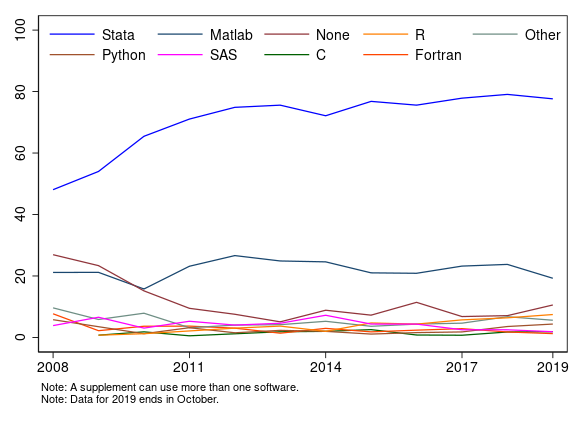
This is not a surprise to anyone who has used Stata. I believe one important reason researchers choose Stata is that reproducing your results is easy. Case in point is the graph above. To get the data and reproduce the graph, you just need to run the do-file, which I discuss in Appendix I. If you want to create a reproducible report, see my discussion in Appendix II.
Appendix I: Explaining the do-file
The do-file below mainly uses three commands: import delimited, which I use to get the comma-separated value dataset used for the graph; xtline, which I use to generate the graph; and egen, which helps me to generate a numeric categorical variable from a string variable using the group function. The other commands I use simplify readability, allow me to modify the code, and help me display results.
Line 1 is there for reproducibility. Stata is the only package I am aware of with integrated version control ensuring that scripts written as long ago as 2008, and indeed, even earlier, can still be used to reproduce their results in the modern version of the software. Lines 5 to 7 create locals for the location of the files. I use them in my call to import delimited. Line 16 creates a categorical variable from a string variable. Each category corresponds to a software package. In the next line, I keep a subset of the data. The data I keep correspond to the time period since the AEA implemented its data policy. In line 21, I use xtset to declare data as a panel and then to be able to use xtline. In line 22, I change the default Stata graphic scheme. Stata has multiple schemes, and you could even write one that best represents your preferences. I like the simplicity of s1color. The remaining code reproduces figure 1.
version 16

// Simplyfing readability and allowing for possibly other data downloads

local  where "https://raw.githubusercontent.com/AEADataEditor"
local  folder "aea-supplement-migration/master/data/generated"
local data "table.aea.software_by_year.csv"

// Importing dataset

import delimited using "`where'/`folder'/`data'",   ///
clear varnames(1) colrange(2:9)

// Generating a numeric variable to graph

egen software_num = group(software_collapsed), label
keep if year > 2007

// Graphing

xtset software_num year
set scheme s1color
xtline percent, overlay legend(position(10) ring(0) rows(2)         ///
   region(lstyle(none)) order(9 3 4 7 5 6 8 1 2))                   ///
   ytitle("") xtitle("") xlabel(2008(3)2017 2019)                   ///
   ylabel(0(20)100)  plotregion(margin(medium))                     ///
   plot9(lcolor(blue))                                              ///
   note("Note: A supplement can be used in more than one software." ///
   "Note: Data for 2019 ends in October.")
Appendix II: Making it a reproducible document
You can create a reproducible report in Word, Excel, PDF, and HTML using Stata. By reproducible, I mean that you can run a do-file that produces Stata results and outputs them into the format you want.
I want to create an HTML document. I save a do-file as a text file and give it the name aea.txt. Then, I type dyndoc “aea.txt”, replace. I generate an HTML document. Aside from aea.txt, I use two other files to produce my HTML document. First, I create a header.txt file. The header.txt file contains HTML code to include at the top of the target HTML file. The header refers to the second file, stmarkdown.css, which is a style sheet that defines how the HTML document is to be formatted.
Now that I have my HTML documents, with Stata’s reporting tools, I can migrate from HTML to Word using one line of code, html2docx aea.html, saving(aea.docx) replace, and from Word to PDF, again, with one line of code, docx2pdf aea.docx, saving (aea.pdf) replace.
Reference
Vilhuber, L., J. Turrito, and K. Welch. 2020. Report by the AEA Data Editor. AEA Papers and Proceedings 110: 764–775. https://doi.org/10.1257/pandp.110.764.