How to create animated choropleth maps using the COVID-19 data from Johns Hopkins University
In my previous posts, I showed how to download the COVID-19 data from the Johns Hopkins GitHub repository, graph the data over time, and create choropleth maps. Now, I’m going to show you how to create animated choropleth maps to explore the distribution of COVID-19 over time and place.
The video below shows the cumulative number of COVID-19 cases per 100,000 population for each county in the United States from January 22, 2020, through April 5, 2020. The map doesn’t change much until mid-March, when the virus starts to spread faster. Then, we can see when and where people are being infected. You can click on the “Play” icon on the video to play it and click on the icon on the bottom right to view the video in full-screen mode.
In my last post, we learned how to create a choropleth map. We will need to learn two additional skills to create an animated map: how to create a map for each date in the dataset and how to combine the collection of maps into a video file.
How to create a map for each date
Let’s begin by importing and describing the raw data from the Johns Hopkins GitHub repository. Note that I imported these data on April 5.
. import delimited https://raw.githubusercontent.com/CSSEGISandData/COVID-19/
> master/csse_covid_19_data/csse_covid_19_time_series/
> time_series_covid19_confirmed_US.csv
(86 vars, 3,253 obs)

. describe

Contains data
  obs:         3,253
 vars:            86
--------------------------------------------------------------------------------
              storage   display    value
variable name   type    format     label      variable label
--------------------------------------------------------------------------------
uid             long    %12.0g                UID
iso2            str2    %9s
iso3            str3    %9s
code3           int     %8.0g
fips            long    %12.0g                FIPS
admin2          str21   %21s                  Admin2
province_state  str24   %24s                  Province_State
country_region  str2    %9s                   Country_Region
lat             float   %9.0g                 Lat
long_           float   %9.0g                 Long_
combined_key    str44   %44s                  Combined_Key
v12             byte    %8.0g                 1/22/20
v13             byte    %8.0g                 1/23/20
v14             byte    %8.0g                 1/24/20
v15             byte    %8.0g                 1/25/20
v16             byte    %8.0g                 1/26/20

               (Output omitted)

v82             long    %12.0g                4/1/20
v83             long    %12.0g                4/2/20
v84             long    %12.0g                4/3/20
v85             long    %12.0g                4/4/20
v86             long    %12.0g                4/5/20
--------------------------------------------------------------------------------
Sorted by:
The variables v12 through v86 contain the cumulative number of confirmed cases of COVID-19 in each county for each day starting on January 22, 2020, and ending on April 5, 2020. Let’s list some observations to view the raw data.
. list combined_key v12 v13 v84 v85 v86 in 6/10

     +----------------------------------------------------+
     |         combined_key   v12   v13   v84   v85   v86 |
     |----------------------------------------------------|
  6. | Autauga, Alabama, US     0     0    12    12    12 |
  7. | Baldwin, Alabama, US     0     0    28    29    29 |
  8. | Barbour, Alabama, US     0     0     1     2     2 |
  9. |    Bibb, Alabama, US     0     0     4     4     5 |
 10. |  Blount, Alabama, US     0     0     9    10    10 |
     +----------------------------------------------------+
We will need to include v12 through v86 in our final dataset. I have copied the code block from the end of my last post and pasted it below with two small modifications. The first modification is displayed in red. The code retains and formats the case data for every date saved in v12 through v86. Note that I refer to “v12 through v86” in the code by typing v*. The asterisk serves as a wildcard, so v* refers to any variable that begins with the letter “v”. The second modification is that we do not create a variable for our population-adjusted count at this point.
// Create the geographic dataset

clear

copy https://www2.census.gov/geo/tiger/GENZ2018/shp/cb_2018_us_county_500k.zip ///

    cb_2018_us_county_500k.zip

unzipfile cb_2018_us_county_500k.zip

spshape2dta cb_2018_us_county_500k.shp, saving(usacounties) replace

use usacounties.dta, clear

generate fips = real(GEOID)

save usacounties.dta, replace
// Create the COVID-19 case dataset

clear

import delimited https://raw.githubusercontent.com/CSSEGISandData/COVID-19/master/csse_covid_19_data/csse_covid_19_time_series/time_series_covid19_confirmed_US.csv

drop if missing(fips)

save covid19_county, replace
// Create the population dataset

clear

import delimited https://www2.census.gov/programs-surveys/popest/datasets/2010-2019/counties/totals/co-est2019-alldata.csv

generate fips = state*1000 + county

save census_popn, replace
// Merge the datasets

clear

use _ID _CX _CY GEOID fips using usacounties.dta

merge 1:1 fips using covid19_county  ///

    , keepusing(province_state combined_key v*)

keep if _merge == 3

drop _merge

merge 1:1 fips using census_popn  ///

    , keepusing(census2010pop popestimate2019)

keep if _merge==3

drop _merge

drop if inlist(province_state, "Alaska", "Hawaii")

format %16.0fc popestimate2019 v*

save covid19_adj, replace
Let’s describe some of our final dataset.
. describe _ID _CX _CY popestimate2019 v*

              storage   display    value
variable name   type    format     label      variable label
--------------------------------------------------------------------------------
_ID             int     %12.0g                Spatial-unit ID
_CX             double  %10.0g                x-coordinate of area centroid
_CY             double  %10.0g                y-coordinate of area centroid
popestimate2019 long    %16.0fc               POPESTIMATE2019
v12             byte    %16.0fc               1/22/20
v13             byte    %16.0fc               1/23/20

               (Output omitted)

v85             long    %16.0fc               4/4/20
v86             long    %16.0fc               4/5/20
The dataset contains all the variables that we will need to create our animated map: the geographic information, the population of each county, and the number of cases for each day in v12 through v86. I am going to explain all the steps we will need to take using only three of these variables. Then, we will put them together using all 75 variables.
We will need to create a separate map for v12, v13, v14, and so forth to v86. Recall that we learned about loops in one of my previous posts. We can use forvalues to loop over the variables.
The forvalues loop below will store the numbers 12, 13, and 14 to the local macro time. You can refer to time inside the loop using left and right single quotes. The example below describes each variable.
. forvalues time = 12/14 {
  2.     describe v`time'
  3. }

              storage   display    value
variable name   type    format     label      variable label
--------------------------------------------------------------------------------
v12             byte    %16.0fc               1/22/20

              storage   display    value
variable name   type    format     label      variable label
--------------------------------------------------------------------------------
v13             byte    %16.0fc               1/23/20

              storage   display    value
variable name   type    format     label      variable label
--------------------------------------------------------------------------------
v14             byte    %16.0fc               1/24/20
We will also need to calculate the population-adjusted number of cases for each county for each day. In the example below, we begin by generating a variable named confirmed_adj that contains missing values. Inside the loop, we replace confirmed_adj with the adjusted count for the current day and summarize confirmed_adj. Then, we drop confirmed_adj when the loop is finished.
. generate confirmed_adj = .
(3,108 missing values generated)

. forvalues time = 12/14 {
  2.     replace confirmed_adj = 100000*(v`time'/popestimate2019)
  3.     summarize confirmed_adj
  4. }
(3,108 real changes made)

    Variable |        Obs        Mean    Std. Dev.       Min        Max
-------------+---------------------------------------------------------
confirmed_~j |      3,108    .0000143    .0007962          0   .0443896
(0 real changes made)

    Variable |        Obs        Mean    Std. Dev.       Min        Max
-------------+---------------------------------------------------------
confirmed_~j |      3,108    .0000143    .0007962          0   .0443896
(1 real change made)

    Variable |        Obs        Mean    Std. Dev.       Min        Max
-------------+---------------------------------------------------------
confirmed_~j |      3,108    .0000205     .000869          0   .0443896

. drop confirmed_adj
We might also wish to include the date in the title of each map. Recall that dates are stored as the number of days since January 1, 1960. The variable v12 contains data for January 22, 2020. We can calculate the number of days since January 1, 1960 using the date() function.
. display date("January 22, 2020", "MDY")
21936
Our forvalues loop begins at time = 12, and we would like the date for v12 to be 21936. So we must subtract 12 from the date before we add the value of the local macro time. The example below loops over the days from January 22, 2020, to January 24, 2020.
. forvalues time = 12/14 {
  2.     display 21936 - 12 + `time'
  3. }
21936
21937
21938
We can then use the string() function to change the display format of each date.
. forvalues time = 12/14 {
  2.     local date = 21936 - 12 + `time'
  3.     display string(`date', "%tdMonth_dd,_CCYY")
  4. }
January 22, 2020
January 23, 2020
January 24, 2020
We will also use graph export to export our graphs to Portable Network Graphics (.png) files. These files will be combined later to create our video, and the filenames must be numbered sequentially from “1” with leading zeros. The example below demonstrates how to use the string() function to create these filenames.
. forvalues time = 12/14 {
  2.     local filenum = string(`time'-11,"%03.0f")
  3.     display "graph export map_`filenum'.png"
  4. }
graph export map_001.png
graph export map_002.png
graph export map_003.png
Let’s put all the pieces together and display the basic commands that we will use to create each map.
. generate confirmed_adj = .
(3,108 missing values generated)

. forvalues time = 12/14 {
  2.     local date    = 21936 - 12 + `time'
  3.     local date    = string(`date', "%tdMonth_dd,_CCYY")
  4.     local filenum = string(`time'-11,"%03.0f")
  5.     display "replace confirmed_adj = 100000*(v`time'/popestimate2019)"
  6.     display "grmap confirmed_adj, title(Map for `date')"
  7.     display "graph export map_`filenum'.png"
  8.     display
  9. }
replace confirmed_adj = 100000*(v12/popestimate2019)
grmap confirmed_adj, title(Map for January 22, 2020)
graph export map_001.png

replace confirmed_adj = 100000*(v13/popestimate2019)
grmap confirmed_adj, title(Map for January 23, 2020)
graph export map_002.png

replace confirmed_adj = 100000*(v14/popestimate2019)
grmap confirmed_adj, title(Map for January 24, 2020)
graph export map_003.png

. drop confirmed_adj
Each iteration of the loop does three things. The first line replaces the variable confirmed_adj with the population-adjusted count for that particular day. The second line uses grmap to create the map with the date in the title. The third line exports the graph to a .png file with sequential filenames starting at 001.
The code block below does the same thing but with some options added to grmap and graph export. Most of the grmap options were discussed in my last post. I have added the option ocolor(gs8) to render the map outline color with light-gray scale and the option osize(vthin) to make the map lines thinner. The options width(3840) and height(2160) after graph export specify that each map be saved at 4K resolution. This will create clear, detailed images for our video.
generate confirmed_adj = .

forvalues time = 12/86 {

    local date = 21936 - 12 + `time'

    local date = string(`date', "%tdMonth_dd,_CCYY")

    replace confirmed_adj = 100000*(v`time'/popestimate2019)

    grmap confirmed_adj,                                                    ///

        clnumber(8)                                                         ///

        clmethod(custom)                                                    ///

        clbreaks(0 5 10 15 20 25 50 100 5000)                               ///

        ocolor(gs8) osize(vthin)                                             ///

        title("Confirmed Cases of COVID-19 in the United States on `date'") ///

        subtitle("cumulative cases per 100,000 population")
    local filenum = string(`time'-11,"%03.0f")

    graph export "map_`filenum'.png", as(png) width(3840) height(2160)

}

drop confirmed_adj
The code block above will create 75 maps and save them in 75 files.
. ls
  <dir>   4/06/20 19:36  .
  <dir>   4/06/20 19:36  ..
1551.2k   4/06/20 10:52  map_001.png
1551.6k   4/06/20 10:52  map_002.png
1550.9k   4/06/20 10:53  map_003.png

    (Output omitted)

1589.1k   4/06/20 11:12  map_073.png
1587.2k   4/06/20 11:13  map_074.png
1585.9k   4/06/20 11:40  map_075.png
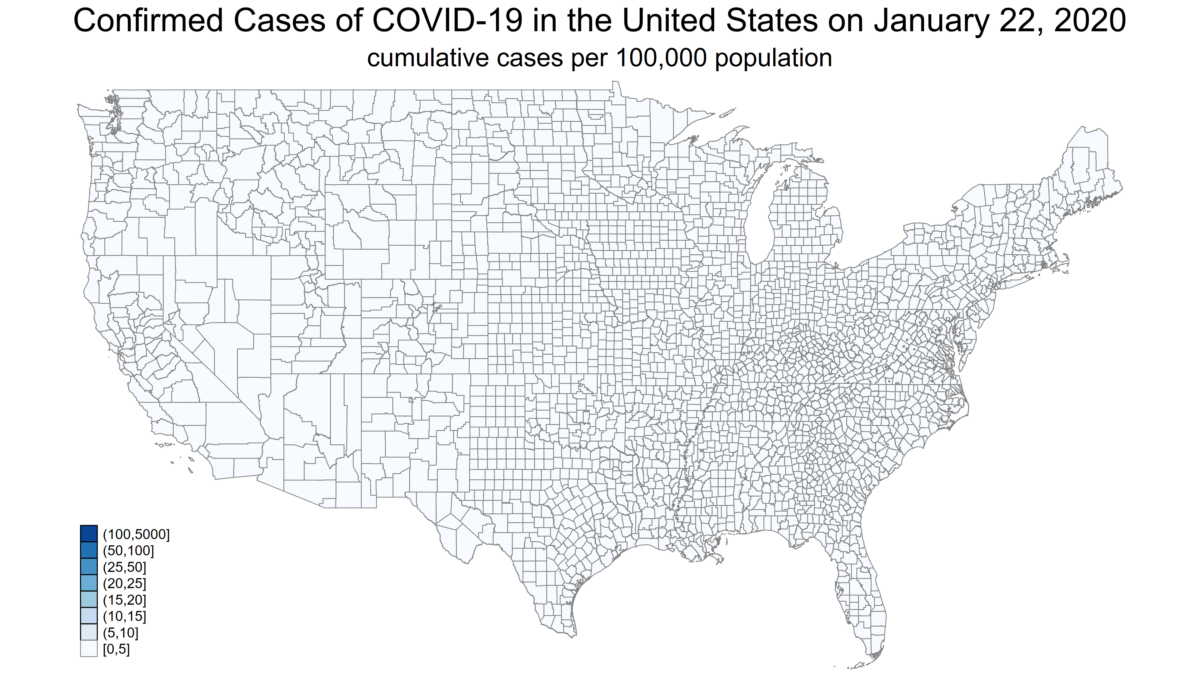
Let’s view the file map_001.png, which is the map for January 22, 2020.
Figure 1: map_001.png
Next, let’s view the file map_075.png, which is the map for April 5, 2020.
Figure 2: map_0075.png
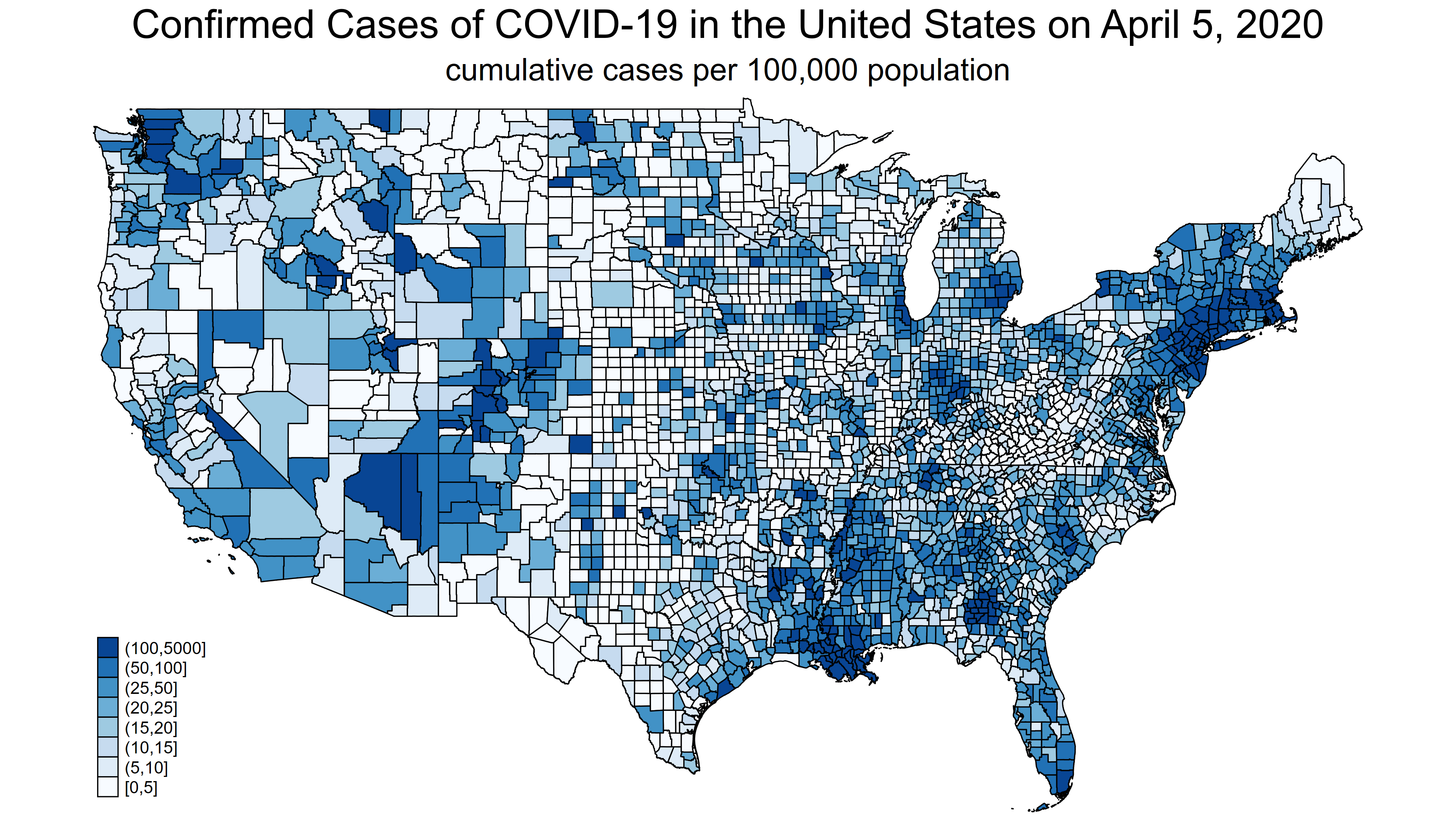
Note that the legend at the bottom left of both maps is the same. I used the clmethod(custom) option with grmap to specify my own cutpoints for values of confirmed_adj. The legend will change from day to day if you use the default clmethod(), which selects the cutpoints based on quantiles of confirmed_adj. The quantiles will change from day to day, and the legend will not be consistent across maps. I selected the cutpoints in clbreaks(0 5 10 15 20 25 50 100 5000) based on the map of the final day.
You can update your video with future data by increasing the upper limit of the forvalues loop. For example, on April 12, 2020, I would type forvalues time = 12/91.
We successfully created a map for each day and saved each map to a separate file. Now, we need to combine these files to create our video.
How to create a video from the collection of maps
I wrote a blog post in 2014 that describes how to use FFmpeg to create a video from a collection of images. FFmpeg is a free software package with versions available for Linux, Mac, and Windows. You can execute FFmpeg commands from within Stata using shell.
The example below uses FFmpeg to combine our map files into a video named covid19.mp4.
shell "ffmpeg.exe" -framerate 1/.5 -i map_%03d.png -c:v libx264 -r 30 -pix_fmt yuv420p covid19.mp4
You may need to specify the location of ffmpeg.exe on your computer as in the example below.
shell "C:\Program Files\ffmpeg\bin\ffmpeg.exe" -framerate 1/.5 -i map_%03d.png -c:v libx264 -r 30 -pix_fmt yuv420p covid19.mp4
The names of the image files are specified with the option -i map_%03d.png, and the name of the output video, covid19.mp4, is specified at the end of the command. The frame rate is specified with the option -framerate 1/.5. The ratio “1/.5” specifies a frame rate of 2 images per second.
FFmpeg may take several minutes to process the images and convert them to a video. Your patience will be rewarded with the video below.
Conclusion and collected code
We did it! We successfully created an animated choropleth map that shows the population-adjusted confirmed cases of COVID-19 for every county in the United State from January 22, 2020, through April 5, 2020. Our video is a powerful tool that we can use to study the distribution of COVID-19 over time and location.
I would like to remind you that I have made somewhat arbitrary decisions while cleaning the data that are used to create this video. My goal was to show you how to create your own maps and videos. My results should be used for educational purposes only, and you will need to check the data carefully if you plan to use the results to make decisions.
You can reproduce the video with the code below.
// Create the geographic dataset

clear

copy https://www2.census.gov/geo/tiger/GENZ2018/shp/cb_2018_us_county_500k.zip ///

    cb_2018_us_county_500k.zip

unzipfile cb_2018_us_county_500k.zip

spshape2dta cb_2018_us_county_500k.shp, saving(usacounties) replace

use usacounties.dta, clear

generate fips = real(GEOID)

save usacounties.dta, replace
// Create the COVID-19 case dataset

clear

import delimited https://raw.githubusercontent.com/CSSEGISandData/COVID-19/master/csse_covid_19_data/csse_covid_19_time_series/time_series_covid19_confirmed_US.csv

drop if missing(fips)

save covid19_county, replace
// Create the population dataset

clear

import delimited https://www2.census.gov/programs-surveys/popest/datasets/2010-2019/counties/totals/co-est2019-alldata.csv

generate fips = state*1000 + county

save census_popn, replace
// Merge the datasets

clear

use _ID _CX _CY GEOID fips using usacounties.dta

merge 1:1 fips using covid19_county  ///

    , keepusing(province_state combined_key v*)

keep if _merge == 3

drop _merge

merge 1:1 fips using census_popn  ///

    , keepusing(census2010pop popestimate2019)

keep if _merge==3

drop _merge

drop if inlist(province_state, "Alaska", "Hawaii")

format %16.0fc popestimate2019 v*

save covid19_adj, replace
// Create the maps

spset, modify shpfile(usacounties_shp)

generate confirmed_adj = .

forvalues time = 12/86 {

    local date = 21936 - 12 + `time'

    local date = string(`date', "%tdMonth_dd,_CCYY")

    replace confirmed_adj = 100000*(v`time'/popestimate2019)

    grmap confirmed_adj,                                                    ///

        clnumber(8)                                                         ///

        clmethod(custom)                                                    ///

        clbreaks(0 5 10 15 20 25 50 100 5000)                               ///

        ocolor(gs8) osize(vthin)                                             ///

        title("Confirmed Cases of COVID-19 in the United States on `date'") ///

        subtitle("cumulative cases per 100,000 population")
    local filenum = string(`time'-11,"%03.0f")

    graph export "map_`filenum'.png", as(png) width(3840) height(2160)

}

drop confirmed_adj
// Create the video with FFmpeg

shell "C:\Program Files\ffmpeg\bin\ffmpeg.exe" -framerate 1/.5 -i map_%03d.png  -c:v libx264 -r 30 -pix_fmt yuv420p covid19.mp4