Customizable tables in Stata 17, part 4: Table of statistical tests
In my last post, I showed you how to use the new and improved table command with the statistic() option to create a classic table 1. In this post, I want to show you how to use the command() option to create a table of statistical tests. Our goal is to create the table in the Microsoft Word document below.
Create the basic table
Let’s begin by typing webuse nhanes2l to open the NHANES dataset, and let’s type describe to examine some of the variables.
. webuse nhanes2l
(Second National Health and Nutrition Examination Survey)

. describe highbp age hgb hct iron albumin vitaminc zinc copper lead
>          height weight bmi bpsystol bpdiast tcresult tgresult hdresult

Variable      Storage   Display    Value
    name         type    format    label      Variable label
-------------------------------------------------------------------------------
highbp          byte    %8.0g               * High blood pressure
age             byte    %9.0g                 Age (years)
hgb             float   %9.0g                 Hemoglobin (g/dL)
hct             float   %9.0g                 Hematocrit (%)
iron            int     %9.0g                 Serum iron (mcg/dL)
albumin         float   %9.0g                 Serum albumin (g/dL)
vitaminc        float   %9.0g                 Serum vitamin C (mg/dL)
zinc            int     %9.0g                 Serum zinc (mcg/dL)
copper          int     %9.0g                 Serum copper (mcg/dL)
lead            byte    %9.0g                 Lead (mcg/dL)
height          float   %9.0g                 Height (cm)
weight          float   %9.0g                 Weight (kg)
bmi             float   %9.0g                 Body mass index (BMI)
bpsystol        int     %9.0g                 Systolic blood pressure
bpdiast         int     %9.0g                 Diastolic blood pressure
tcresult        int     %9.0g                 Serum cholesterol (mg/dL)
tgresult        int     %9.0g                 Serum triglycerides (mg/dL)
hdresult        int     %9.0g                 High density lipids (mg/dL)
The dataset includes an indicator for high blood pressure (highbp), age, and many lab measurements. We would like to test the null hypothesis that the average age and lab measurments are the same in the groups with and without, hypertension. We can do this with Stata’s ttest command. Let’s use ttest to test the null hypothesis that the average age is the same in the two groups.
. ttest age, by(highbp)

Two-sample t test with equal variances
------------------------------------------------------------------------------
   Group |     Obs        Mean    Std. err.   Std. dev.   [95% conf. interval]
---------+--------------------------------------------------------------------
       0 |   5,975    42.16502    .2169725    16.77157    41.73968    42.59037
       1 |   4,376    54.97281    .2253767    14.90897    54.53095    55.41466
---------+--------------------------------------------------------------------
Combined |  10,351    47.57965    .1692044    17.21483    47.24798    47.91133
---------+--------------------------------------------------------------------
    diff |           -12.80779    .3185604               -13.43223   -12.18335
------------------------------------------------------------------------------
    diff = mean(0) - mean(1)                                      t = -40.2052
H0: diff = 0                                     Degrees of freedom =    10349

    Ha: diff < 0                 Ha: diff != 0                 Ha: diff > 0
 Pr(T < t) = 0.0000         Pr(|T| > |t|) = 0.0000          Pr(T > t) = 1.0000
The output displays many statistics, including the two-sided p-value for the t test. Some of these statistics are temporarily left in memory and we can view them by typing return list.
. return list

scalars:
              r(level) =  95
                 r(sd) =  17.21482923023818
               r(sd_2) =  14.9089715191102
               r(sd_1) =  16.77156676799842
                 r(se) =  .3185603831285
                r(p_u) =  1
                r(p_l) =  0
                  r(p) =  0
                  r(t) =  -40.20520433030012
               r(df_t) =  10349
               r(mu_2) =  54.97280621572212
                r(N_2) =  4376
               r(mu_1) =  42.16502092050209
                r(N_1) =  5975
We can use the command() option in table to run a command, such as ttest, and put the results in a table. The example below shows the basic syntax for creating a table of results from ttest. The row dimension is command, the column dimension is result, and we place our ttest command in the command() option.
. table (command) (result),
>       command(ttest age, by(highbp))
(output omitted)
I omitted the output because table tried to include all the results in the table and the output doesn’t fit on the screen. Let’s be more specific in command() about the statistics we wish to include in our table. Let’s add a column named Normotensive for the mean age of people without hypertension, which is stored in the scalar r(mu_1) by ttest. We can also add a column named Hypertensive for the mean age of people with hypertension, which is stored in the scalar r(mu_2), a column named Diff for the difference between the group means, and a column named pvalue that displays the p-value stored in r(p).
. table (command) (result),
>       command(Normotensive = r(mu_1)
>               Hypertensive = r(mu_2)
>               Diff         = (r(mu_2)-r(mu_1))
>               pvalue       =  r(p)
>               : ttest age, by(highbp))

------------------------------------------------------------------------
                      |  Normotensive   Hypertensive       Diff   pvalue
----------------------+-------------------------------------------------
ttest age, by(highbp) |      42.16502       54.97281   12.80779        0
------------------------------------------------------------------------
The output displays the ttest command in the first column, followed by the means, difference, and p-value that we specified in our table command. I would like to replace the command name in the table with the label Age (years). Recall that dimensions have levels and levels can have labels. Let’s type collect label list command, all to view the levels and labels of the dimension command.
. collect label list command, all

  Collection: Table
   Dimension: command
       Label: Command option index
Level labels:
           1  ttest age, by(highbp)
The output tells us that the dimension command has one level, 1, which is labeled ttest age, by(highbp). We can change the label for level 1 using collect label levels. Then we can type collect preview to view our updated table.
. collect label levels command 1 "Age (years)", modify

. collect preview

--------------------------------------------------------------
            |  Normotensive   Hypertensive       Diff   pvalue
------------+-------------------------------------------------
Age (years) |      42.16502       54.97281   12.80779        0
--------------------------------------------------------------
Next we can use collect style cell to change the number of decimals displayed in each cell and remove the right border from the first column.
. collect style cell result[Normotensive Hypertensive Diff],
>         nformat(%6.1f)

. collect style cell result[pvalue], nformat(%6.4f)

. collect style cell border_block, border(right, pattern(nil))

. collect preview

--------------------------------------------------------
             Normotensive   Hypertensive   Diff   pvalue
--------------------------------------------------------
Age (years)          42.2           55.0   12.8   0.0000
--------------------------------------------------------
We did it! Our table looks good, but we have only included a test for one variable. Let’s add more.
Create a larger table
The obvious way to add more tests to our table would be to add more command() options. That would work as we can see below.
. table (command) (result),
>       command(Normotensive = r(mu_1) Hypertensive = r(mu_2)
>               Diff = (r(mu_2)-r(mu_1)) pvalue = r(p)
>               : ttest age, by(highbp))
>       command(Normotensive = r(mu_1) Hypertensive = r(mu_2)
>               Diff = (r(mu_2)-r(mu_1)) pvalue = r(p)
>               : ttest tcresult, by(highbp))
>       command(Normotensive = r(mu_1) Hypertensive = r(mu_2)
>               Diff = (r(mu_2)-r(mu_1)) pvalue = r(p)
>               : ttest tgresult, by(highbp))
>       command(Normotensive = r(mu_1) Hypertensive = r(mu_2)
>               Diff = (r(mu_2)-r(mu_1)) pvalue = r(p)
>               : ttest hdresult, by(highbp))
>       nformat(%6.2f  Normotensive Hypertensive Diff)
>       nformat(%6.4f  pvalue)

--------------------------------------------------------------------------
                           |  Normotensive   Hypertensive    Diff   pvalue
---------------------------+----------------------------------------------
ttest age, by(highbp)      |         42.17          54.97   12.81   0.0000
ttest tcresult, by(highbp) |        208.73         229.88   21.15   0.0000
ttest tgresult, by(highbp) |        129.23         166.04   36.81   0.0000
ttest hdresult, by(highbp) |         49.94          49.22   -0.73   0.0195
--------------------------------------------------------------------------
But our table command is growing faster than our table. Fortunately, we can use a little programming trick to make our task easier and our code neater. Notice that most of the code in our command() options is identical. We can store that code in a local macro and use the local macro in our command() options. I have stored the commands in a local macro named myresults.
. local myresults "Normotensive = r(mu_1) Hypertensive = r(mu_2) Diff = (r(mu_2)-r(mu_1)) pvalue = r(p)"

. display "`myresults'"
Normotensive = r(mu_1) Hypertensive = r(mu_2)  Diff = (r(mu_2)-r(mu_1))  pvalue = r(p)
Now we can replace the lengthy column definitions with the local macro `myresults’ in our command() options.
. table (command) (result),
>       command(`myresults' : ttest age,      by(highbp))
>       command(`myresults' : ttest tcresult, by(highbp))
>       command(`myresults' : ttest tgresult, by(highbp))
>       command(`myresults' : ttest hdresult, by(highbp))
>       nformat(%6.2f  Normotensive Hypertensive Diff)
>       nformat(%6.0f  pvalue)

--------------------------------------------------------------------------
                           |  Normotensive   Hypertensive    Diff   pvalue
---------------------------+----------------------------------------------
ttest age, by(highbp)      |         42.17          54.97   12.81        0
ttest tcresult, by(highbp) |        208.73         229.88   21.15        0
ttest tgresult, by(highbp) |        129.23         166.04   36.81        0
ttest hdresult, by(highbp) |         49.94          49.22   -0.73        0
--------------------------------------------------------------------------
Let’s add the rest of the lab variables to our table using our clever new trick.
. table (command) (result),
>       command(`myresults' : ttest age,      by(highbp))
>       command(`myresults' : ttest hgb,      by(highbp))
>       command(`myresults' : ttest hct,      by(highbp))
>       command(`myresults' : ttest iron,     by(highbp))
>       command(`myresults' : ttest albumin,  by(highbp))
>       command(`myresults' : ttest vitaminc, by(highbp))
>       command(`myresults' : ttest zinc,     by(highbp))
>       command(`myresults' : ttest copper,   by(highbp))
>       command(`myresults' : ttest lead,     by(highbp))
>       command(`myresults' : ttest height,   by(highbp))
>       command(`myresults' : ttest weight,   by(highbp))
>       command(`myresults' : ttest bmi,      by(highbp))
>       command(`myresults' : ttest bpsystol, by(highbp))
>       command(`myresults' : ttest bpdiast,  by(highbp))
>       command(`myresults' : ttest tcresult, by(highbp))
>       command(`myresults' : ttest tgresult, by(highbp))
>       command(`myresults' : ttest hdresult, by(highbp))
--------------------------------------------------------------------------------
                           |  Normotensive   Hypertensive        Diff     pvalue
---------------------------+----------------------------------------------------
ttest age, by(highbp)      |      42.16502       54.97281    12.80779          0
ttest height, by(highbp)   |      167.7243       167.5506   -.1736495   .3661002
ttest weight, by(highbp)   |      68.26626       76.85565    8.589386   9.1e-181
ttest bmi, by(highbp)      |      24.20231       27.36081    3.158506   4.5e-241
ttest bpsystol, by(highbp) |       116.485       150.5388    34.05383          0
ttest bpdiast, by(highbp)  |      74.17222       92.01394    17.84172          0
ttest tcresult, by(highbp) |      208.7272       229.8798     21.1526   4.3e-105
ttest tgresult, by(highbp) |      129.2284       166.0427     36.8143   7.01e-41
ttest hdresult, by(highbp) |      49.94449       49.21784   -.7266526   .0194611
ttest hgb, by(highbp)      |      14.14038       14.42436    .2839752   4.99e-25
ttest hct, by(highbp)      |      41.65235       42.44271    .7903588   2.16e-27
ttest iron, by(highbp)     |       101.842       96.17436   -5.667648   5.70e-17
ttest albumin, by(highbp)  |      4.680295       4.654088   -.0262068   .0000896
ttest vitaminc, by(highbp) |      1.048238       1.016469   -.0317686   .0070212
ttest zinc, by(highbp)     |      87.06462       85.74782   -1.316802   .0000162
ttest copper, by(highbp)   |      125.0756       126.3356    1.259952   .0673572
ttest lead, by(highbp)     |      13.87513       14.93369    1.058555   2.36e-09
--------------------------------------------------------------------------------
Next we can change the labels of the levels of the dimension command. Let’s begin by listing the labels for each level.
. collect label list command, all

  Collection: Table
   Dimension: command
       Label: Command option index
Level labels:
           1  ttest age, by(highbp)
          10  ttest height, by(highbp)
          11  ttest weight, by(highbp)
          12  ttest bmi, by(highbp)
          13  ttest bpsystol, by(highbp)
          14  ttest bpdiast, by(highbp)
          15  ttest tcresult, by(highbp)
          16  ttest tgresult, by(highbp)
          17  ttest hdresult, by(highbp)
           2  ttest hgb, by(highbp)
           3  ttest hct, by(highbp)
           4  ttest iron, by(highbp)
           5  ttest albumin, by(highbp)
           6  ttest vitaminc, by(highbp)
           7  ttest zinc, by(highbp)
           8  ttest copper, by(highbp)
           9  ttest lead, by(highbp)
Notice that the levels are sorted as strings rather than numbers. This is because levels can be strings or numbers. We can see the variable names associated with each level, and we can relabel them using collect label levels.
. collect label levels command 1  "Age (years)"
>                              10 "Height (cm)"
>                              11 "Weight (kg)"
>                              12 "Body Mass Index"
>                              13 "Systolic Blood Pressure"
>                              14 "Diastolic Blood Pressure"
>                              15 "Serum cholesterol (mg/dL)"
>                              16 "Serum triglycerides (mg/dL)"
>                              17 "High density lipids (mg/dL)"
>                              2  "Hemoglobin (g/dL)"
>                              3  "Hematocrit (%)"
>                              4  "Serum iron (mcg/dL)"
>                              5  "Serum albumin (g/dL)"
>                              6  "Serum vitamin C (mg/dL)"
>                              7  "Serum zinc (mcg/dL)"
>                              8  "Serum copper (mcg/dL)"
>                              9 "Lead (mcg/dL)"
>                              , modify

. collect preview

---------------------------------------------------------------------------------
                            |  Normotensive   Hypertensive        Diff     pvalue
----------------------------+----------------------------------------------------
Age (years)                 |      42.16502       54.97281    12.80779          0
Height (cm)                 |      167.7243       167.5506   -.1736495   .3661002
Weight (kg)                 |      68.26626       76.85565    8.589386   9.1e-181
Body Mass Index             |      24.20231       27.36081    3.158506   4.5e-241
Systolic Blood Pressure     |       116.485       150.5388    34.05383          0
Diastolic Blood Pressure    |      74.17222       92.01394    17.84172          0
Serum cholesterol (mg/dL)   |      208.7272       229.8798     21.1526   4.3e-105
Serum triglycerides (mg/dL) |      129.2284       166.0427     36.8143   7.01e-41
High density lipids (mg/dL) |      49.94449       49.21784   -.7266526   .0194611
Hemoglobin (g/dL)           |      14.14038       14.42436    .2839752   4.99e-25
Hematocrit (%)              |      41.65235       42.44271    .7903588   2.16e-27
Serum iron (mcg/dL)         |       101.842       96.17436   -5.667648   5.70e-17
Serum albumin (g/dL)        |      4.680295       4.654088   -.0262068   .0000896
Serum vitamin C (mg/dL)     |      1.048238       1.016469   -.0317686   .0070212
Serum zinc (mcg/dL)         |      87.06462       85.74782   -1.316802   .0000162
Serum copper (mcg/dL)       |      125.0756       126.3356    1.259952   .0673572
Lead (mcg/dL)               |      13.87513       14.93369    1.058555   2.36e-09
---------------------------------------------------------------------------------
Finally, let’s format the numbers using collect style cell and remove the right border from the first column.
. collect style cell result[Normotensive Hypertensive Diff], nformat(%8.2f)
. collect style cell result[pvalue], nformat(%6.4f)
. collect style cell border_block, border(right, pattern(nil))
. collect preview
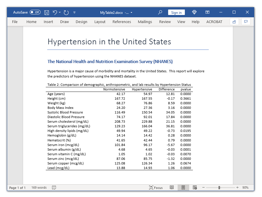
-------------------------------------------------------------------------
Normotensive Hypertensive Diff pvalue
-------------------------------------------------------------------------
Age (years) 42.17 54.97 12.81 0.0000
Height (cm) 167.72 167.55 -0.17 0.3661
Weight (kg) 68.27 76.86 8.59 0.0000
Body Mass Index 24.20 27.36 3.16 0.0000
Systolic Blood Pressure 116.49 150.54 34.05 0.0000
Diastolic Blood Pressure 74.17 92.01 17.84 0.0000
Serum cholesterol (mg/dL) 208.73 229.88 21.15 0.0000
Serum triglycerides (mg/dL) 129.23 166.04 36.81 0.0000
High density lipids (mg/dL) 49.94 49.22 -0.73 0.0195
Hemoglobin (g/dL) 14.14 14.42 0.28 0.0000
Hematocrit (%) 41.65 42.44 0.79 0.0000
Serum iron (mcg/dL) 101.84 96.17 -5.67 0.0000
Serum albumin (g/dL) 4.68 4.65 -0.03 0.0001
Serum vitamin C (mg/dL) 1.05 1.02 -0.03 0.0070
Serum zinc (mcg/dL) 87.06 85.75 -1.32 0.0000
Serum copper (mcg/dL) 125.08 126.34 1.26 0.0674
Lead (mcg/dL) 13.88 14.93 1.06 0.0000
-------------------------------------------------------------------------
Export the table to Microsoft Word
Once we’re happy with the layout of our table, we can export it to many different file formats. I’m going to use putdocx, collect style putdocx, and putdocx collect to export our table to a Microsoft Word document. Many of you will notice that the commands below are almost identical to the commands in my previous posts about tables.
. putdocx clear

. putdocx begin

. putdocx paragraph, style(Title)

. putdocx text ("Hypertension in the United States")

. putdocx paragraph, style(Heading1)

. putdocx text ("The National Health and Nutrition Examination Survey (NHANES)")

. putdocx paragraph

. putdocx text ("Hypertension is a major cause of morbidity and mortality in ")

. putdocx text ("the United States.  This report will explore the predictors ")

. putdocx text ("of hypertension using the NHANES dataset.")

. collect style putdocx, layout(autofitcontents)
>         title("Table 2: Comparison of demographic, anthropometric, and lab results by Hypertension Status")

. putdocx collect
(collection Table posted to putdocx)

. putdocx save MyTable2.docx, replace
successfully replaced "MyTable2.docx"
Conclusion
In this post, we learned how to use the command() option with the table command to create a table of statistical tests. The steps are simple: run the command of interest, type return list to view the statistics left in memory, create your table using the row dimension command and the column dimension result, and place your command in the command() option. You may wish to specify custom columns for the statistics in your table, and we learned how to use local macros to simplify that task.
I will show you how to use the command() option to create a table of regression coefficients in my next post.