Importing data with import fred
Introduction
The Federal Reserve Economic Database (FRED), maintained by the Federal Reserve Bank of St. Louis, makes available hundreds of thousands of time-series measuring economic and social outcomes. The new Stata 15 command import fred imports data from this repository.
In this post, I show how to use import fred to import data from FRED. I also discuss some of the metadata that import fred provides that can be useful in data management. I then demonstrate how to use an advanced feature: importing multiple revisions of series whose observations are updated over time.
New data releases update nearly all the series in FRED. For some series, a new data release simply adds observations. For other series, a new data release can change the values of previously released observations, because the values of the observations are estimated or calculated. These changes are made as as the source information changes or as the formulas or methods change. For example, the data on real Gross National Product (GNP) in a specific quarter is updated several times as more complete source information becomes available.
A revision of the data is known as a vintage. Vintages are identified by the date of their release; we speak of “the July 10, 2017 vintage”. The vintage() option in import fred allows you to access earlier vintages of the data.
Prior vintages of data have several uses. First, importing vintage data allows you to view a dataset exactly as it would have been seen in an earlier paper, which is useful for replication purposes. Second, prior vintages can be used as a robustness check; in some contexts, it is useful to investigate whether your results are robust across different vintages of the data. Third, in some applied work, it is necessary to condition on information as it was available in real time, rather than use revised data.
In the example discussed below, later data vintages reveal a deeper recession in 2008 than the earlier vintages.
Using import fred
Like nearly all commands, you can access import fred through a menu-driven graphical user interface (GUI) and through a command-line interface. The FRED repository is best explored using the GUI available from the menu File > Import > Federal Reserve Economic Data (FRED). See [D] import fred, The FRED interface for an introduction to exploring FRED via the import fred GUI. Reproducible tasks are easier using command-line interface. In this post, I use the command-line interface because applications of different vintages almost always have to reproducible.
Before you can reproduce what I do here, you need a key to use FRED, which is freely available from
https://research.stlouisfed.org/docs/api/api_key.html
Click on the link above, select Request or view your API keys, then register to obtain a key. Then, in Stata, type
. set fredkey key, permanently
to set your key.
Series in FRED are identified by an alphanumeric code. FRED codes can be obscure; the import fred GUI and the fredsearch command can greatly help to find the codes for the series you want. To find the code for real GNP, I use fredsearch. This command takes a list of keywords and searches for FRED series matching those keywords. In addition, series in FRED have tags for country, region, etc., and fredsearch can restrict the search to series matching those tags. Below, I use fredsearch to find the series with keywords real, gross, national, and product. I add the option tags(usa) to restrict the search to U.S. data series.
. fredsearch real gross national product, tags(usa)
--------------------------------------------------------------------------------
Series ID          Title                  Data range                Frequency
--------------------------------------------------------------------------------
GNPC96             Real Gross Nationa...  1947-01-01 to 2017-01-01  Quarterly
GNPCA              Real Gross Nationa...  1929-01-01 to 2016-01-01  Annual
Q0896AUSQ240SNBR   Gross National Pro...  1921-01-01 to 1939-10-01  Quarterly
A001RO1Q156NBEA    Real Gross Nationa...  1948-01-01 to 2017-01-01  Quarterly
A791RX0Q048SBEA    Real gross nationa...  1947-01-01 to 2017-01-01  Quarterly
A001RL1A225NBEA    Real Gross Nationa...  1930-01-01 to 2016-01-01  Annual
A001RL1Q225SBEA    Real Gross Nationa...  1947-04-01 to 2017-01-01  Quarterly
Q0896BUSQ008SNBR   Gross National Pro...  1947-01-01 to 1965-10-01  Quarterly
CB22RX1A020NBEA    Command-basis real...  1929-01-01 to 2016-01-01  Annual
Q08321USQ008SNBR   Gross National Pro...  1947-01-01 to 1966-07-01  Quarterly
Q08328USQ350SNBR   Index of Labor Cos...  1948-01-01 to 1966-10-01  Quarterly
Q08300USQ259SNBR   Labor Cost Per Dol...  1947-01-01 to 1966-07-01  Quarterly
B001RA3A086NBEA    Real gross nationa...  1929-01-01 to 2016-01-01  Annual
CB22RX1Q020SBEA    Command-basis real...  1947-01-01 to 2017-01-01  Quarterly
B001RA3Q086SBEA    Real gross nationa...  1947-01-01 to 2017-01-01  Quarterly
--------------------------------------------------------------------------------
Total: 15
The first result is the one we want; the FRED code is GNPC96. I use import fred to import it.
. import fred GNPC96

Summary
--------------------------------------------------------------------------------
Series ID                    Nobs    Date range                Frequency
--------------------------------------------------------------------------------
GNPC96                       281     1947-01-01 to 2017-01-01  Quarterly
--------------------------------------------------------------------------------
# of series imported: 1
   highest frequency: Quarterly
    lowest frequency: Quarterly
The summary table reports the number of series imported and the highest and lowest frequency of the imported series. The first few observations are
. list in 1/8, separator(4)

     +---------------------------------+
     | datestr          daten   GNPC96 |
     |---------------------------------|
  1. | 1947-01-01   01jan1947     1947 |
  2. | 1947-04-01   01apr1947   1945.3 |
  3. | 1947-07-01   01jul1947   1943.3 |
  4. | 1947-10-01   01oct1947   1974.3 |
     |---------------------------------|
  5. | 1948-01-01   01jan1948   2004.2 |
  6. | 1948-04-01   01apr1948   2037.2 |
  7. | 1948-07-01   01jul1948   2048.6 |
  8. | 1948-10-01   01oct1948   2050.8 |
     +---------------------------------+
datestr is a string variable containing the observation date. daten is the Stata daily date variable corresponding to the string date in datestr. By FRED convention, observation dates are stored as daily dates. For example, the date for the first quarter of 1947 is recorded as January 1, 1947.
We now use qofd() to create a quarterly date from daten, and then tsset the dataset:
. generate dateq = qofd(daten)

. tsset dateq, quarterly
        time variable:  dateq, 1947q1 to 2017q1
                delta:  1 quarter
import fred can import multiple series at once and can import series of different frequencies. It can aggregate high-frequency series into a desired lower frequency and can import data over a requested date range. For a full description of the capabilities of import fred, see http://www.stata.com/manuals/dimportfred.pdf.
Importing and inspecting vintages of a series
Having provided the essential background material, I now illustrate how to import and plot several vintages of the GNPC96 series. Updates to this series are particularly interesting because they reveal a lower trough of the Great Recession than those seen in the earlier data releases.
We can import multiple vintages of real GNP with a single import fred command by specifying the series’ FRED code and the desired vintages:
. import fred GNPC96, vintage(2009-04-15 2010-04-15 2011-04-15 2017-04-15) clear

Summary
--------------------------------------------------------------------------------
Series ID                    Nobs    Date range                Frequency
--------------------------------------------------------------------------------
GNPC96_20090415              248     1947-01-01 to 2008-10-01  Quarterly
GNPC96_20100415              252     1947-01-01 to 2009-10-01  Quarterly
GNPC96_20110415              256     1947-01-01 to 2010-10-01  Quarterly
GNPC96_20170415              280     1947-01-01 to 2016-10-01  Quarterly
--------------------------------------------------------------------------------
# of series imported: 4
   highest frequency: Quarterly
    lowest frequency: Quarterly
. generate dateq = qofd(daten)

. tsset dateq, quarterly
        time variable:  dateq, 1947q1 to 2016q4
                delta:  1 quarter
The first command above imports four time series, one for each date specified. The name of each series includes its FRED code and the date requested, so GNPC96_20090415 is the GNPC96 series as it would have been seen on April 15, 2009. The remaining commands generate the quarterly variable and specify it as the tsset variable.
FRED series contain metadata about the series, including the data source, series title, frequency, units, and notes. import fred gives you access to this metadata. Metadata about each imported series is stored in the variable characteristics. Characteristics are similar to notes, but are primarily meant for use in programming contexts. In the case of import fred, the characteristics can contain information that is valuable in data management. Characteristics are viewed with char list and are referred to by varname[charname]. Two characteristics are of primary interest when working with vintages. The characteristic stored in Last_Updated contains the vintage date corresponding to the vintage you imported.
. char list GNPC96_20090415[Last_Updated]
  GNP~20090415[Last_Updated]: 2009-03-26 10:16:11-05

. char list GNPC96_20100415[Last_Updated]
  GNP~20100415[Last_Updated]: 2010-03-26 13:31:07-05

. char list GNPC96_20110415[Last_Updated]
  GNP~20110415[Last_Updated]: 2011-03-25 11:46:13-05

. char list GNPC96_20170415[Last_Updated]
  GNP~20170415[Last_Updated]: 2017-03-30 08:01:04-05
The actual vintage date associated with GNPC96_20090415 is March 26, 2009. When you specify a date that is not a true vintage date, import fred imports the vintage immediately prior to the date requested.
The characteristic Units contains the units that the series is measured in. This characteristic is useful for series whose units may change over time. For example, some series are adjusted for inflation and indexed to a base year; the base year can change over time. Other series have units that do not change over time. I list the units for the four vintages I imported.
. char list GNPC96_20090415[Units]
  GNP~20090415[Units]:        Billions of Chained 2000 Dollars

. char list GNPC96_20100415[Units]
  GNP~20100415[Units]:        Billions of Chained 2005 Dollars

. char list GNPC96_20110415[Units]
  GNP~20110415[Units]:        Billions of Chained 2005 Dollars

. char list GNPC96_20170415[Units]
  GNP~20170415[Units]:        Billions of Chained 2009 Dollars
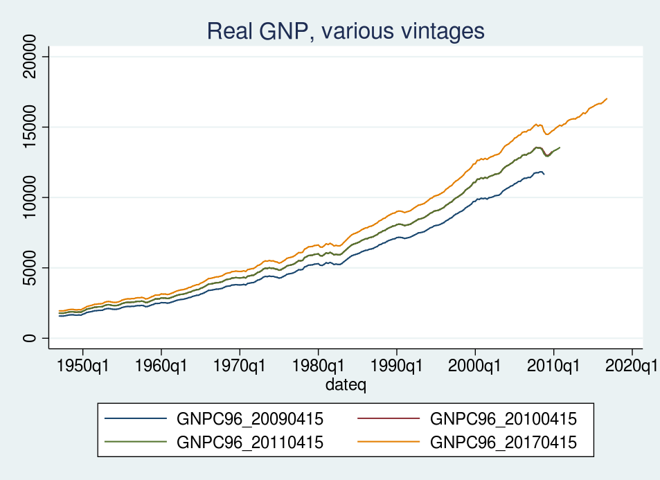
The units are not comparable across all vintages. One of the vintages uses a price index measured in year 2000 dollars; two others use year 2005 dollars; and one uses year 2009 dollars. The difference in base year appears as level shifts in GNP. We can see these level shifts by graphing the series:
. tsline GNPC96*, title("Real GNP, various vintages")
Revisions to the GNP growth rate
In this section, I illustrate that the revisions to GNP in these vintages yield surprisingly different growth rates. The next few graphs plot real GNP growth across the 2009, 2010, 2011, and 2017 vintages. GNP data are often reported in growth rates, and by using growth rates we remove the level shifts caused by the change in base year across vintages.
The growth rate for each vintage is calculated as the quarter-over-quarter percentage change in real GNP. I label each vintage with the year of that vintage.
. generate growth_2009 = 100*(GNPC96_20090415 / L.GNPC96_20090415 - 1)
(33 missing values generated)

. label variable growth_2009 "2009"

. generate growth_2010 = 100*(GNPC96_20100415 / L.GNPC96_20100415 - 1)
(29 missing values generated)

. label variable growth_2010 "2010"

. generate growth_2011 = 100*(GNPC96_20110415 / L.GNPC96_20110415 - 1)
(25 missing values generated)

. label variable growth_2011 "2011"

. generate growth_2017 = 100*(GNPC96_20170415 / L.GNPC96_20170415 - 1)
(1 missing value generated)

. label variable growth_2017 "2017"
The missing values for prior vintages occur because, for example, observations in 2015 do not exist for the 2009 vintage.
I next graph the growth rates calculated from each vintage. First, I graph the 2009 and 2010 vintages together. After that, I graph all four vintages together.
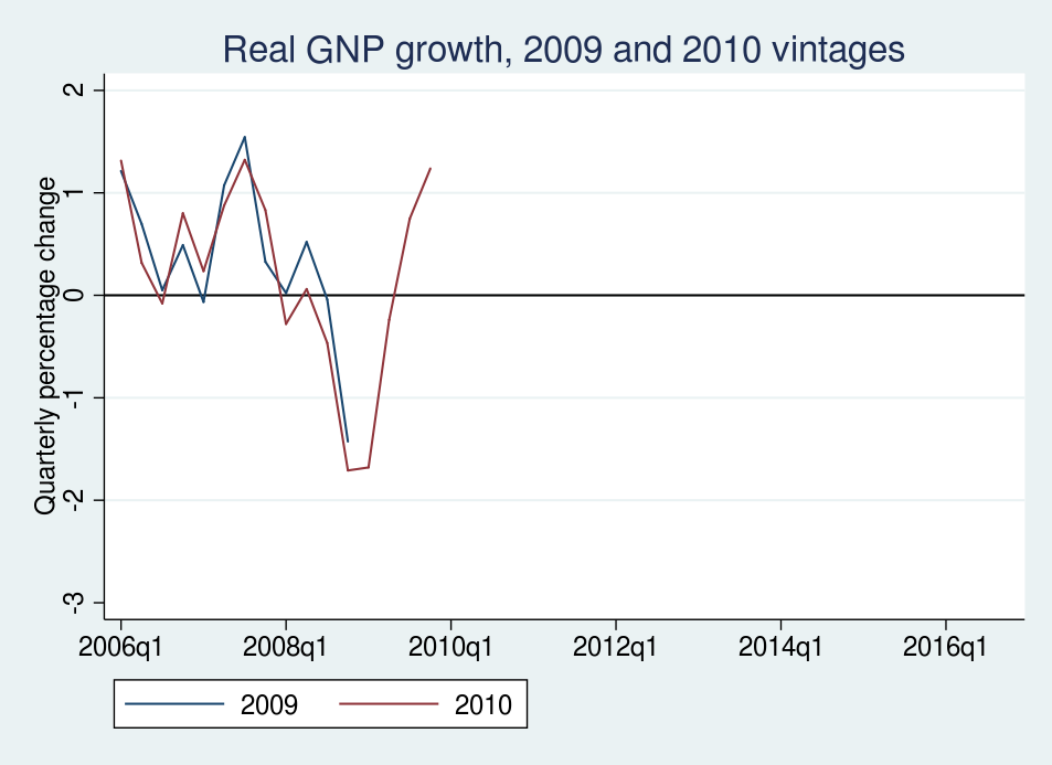
This graph plots the April 15, 2009 and April 15, 2010 vintages of real GNP growth for each quarter starting from the first quarter of 2006. Units are in quarterly percentage change, so a value of 2 indicates 2% growth, quarter over quarter. Most of the revisions are small and uninteresting, especially in 2006 and 2007. Both vintages show that real GNP growth slowed in 2008, but the 2010 vintage indicates that growth slipped into negative territory two quarters earlier than was estimated in the 2009 vintage. The most noticeable revisions are to the observations in the second and fourth quarters of 2008. The 2009 vintage reports that real GNP fell by about 1.5% in the fourth quarter of 2008; the 2010 vintage reports a fall of 1.7%.
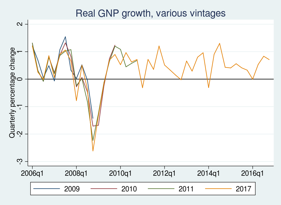
This graph adds the April 15, 2011 and April 15, 2017 vintages of real GNP growth for each quarter starting from the first quarter of 2006. As before, the revisions to observations in 2006 and 2007 are minor. The 2011 and 2017 vintages report a reduction in GNP growth during 2008, relative to the 2009 vintage. Most dramatic are the revisions to the observation in 2008q4. While the 2009 vintage reports a decline in GNP growth of 1.5% in that quarter, the 2017 vintage reports a decline in GNP growth of nearly 3%.
Conclusion
In this post, I demonstrated how to use import fred and how to import multiple vintages of a series. I explored the revisions in real GNP around 2008. Most revisions were unremarkable, but the revisions in some quarters were quantitatively large and revealed a deeper recession trough than the earlier data releases.