Stata/Python integration part 7: Machine learning with support vector machines
Machine learning, deep learning, and artificial intelligence are a collection of algorithms used to identify patterns in data. These algorithms have exotic-sounding names like “random forests”, “neural networks”, and “spectral clustering”. In this post, I will show you how to use one of these algorithms called a “support vector machines” (SVM). I don’t have space to explain an SVM in detail, but I will provide some references for further reading at the end. I am going to give you a brief introduction and show you how to implement an SVM with Python.
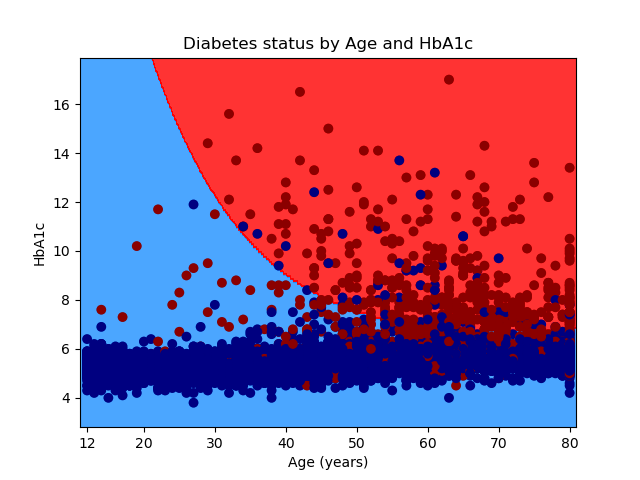
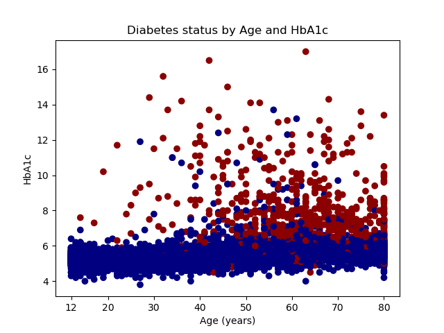
Our goal is to use an SVM to differentiate between people who are likely to have diabetes and those who are not. We will use age and HbA1c level to differentiate between people with and without diabetes. Age is measured in years, and HbA1c is a blood test that measures glucose control. The graph below displays diabetics with red dots and nondiabetics with blue dots. An SVM model predicts that older people with higher levels of HbA1c in the red-shaded area of the graph are more likely to have diabetes. Younger people with lower HbA1c levels in the blue-shaded area are less likely to have diabetes.
If you are not familiar with Python, it may be helpful to read the first four posts in my Stata/Python integration series before you read further.
- Setting up Stata to use Python
- Three ways to use Python in Stata
- How to install Python packages
- How to use Python packages
Download, merge, and clean the data
We will be using data from the United States National Health and Nutrition Examination Survey (NHANES). Specifically, we will be using the variables age from the demographic data,
HbA1c from the glycohemoglobin data, and diabetes from the diabetes data.
The code block below imports three SAS Transport files from the NHANES website,
saves the files to Stata datasets, merges the Stata datasets, renames and recodes the variables, keeps the variables diabetes, age, and HbA1c, drops observations with missing values, and saves the variables to a dataset named diabetes.dta. The last two lines of the code block erase the temporary datasets age.dta and glucose.dta.
import sasxport5 "https://wwwn.cdc.gov/Nchs/Nhanes/2015-2016/DEMO_I.XPT", clear
save age.dta, replace
import sasxport5 "https://wwwn.cdc.gov/Nchs/Nhanes/2015-2016/GHB_I.XPT", clear
save glucose.dta, replace
import sasxport5 "https://wwwn.cdc.gov/Nchs/Nhanes/2015-2016/DIQ_I.XPT", clear
save diabetes, replace

merge 1:1 seqn using "glucose.dta"
drop _merge
merge 1:1 seqn using "age.dta"

rename ridageyr age
rename lbxgh HbA1c
rename diq010 diabetes
recode diabetes (1 = 1) (2/3 = 0) (9=.)

keep diabetes age HbA1c
drop if missing(diabetes, age, HbA1c)
save diabetes, replace

erase age.dta
erase glucose.dta
Let’s list the first five observations in the dataset to check our work.
. list in 1/5

     +------------------------+
     | diabetes   HbA1c   age |
     |------------------------|
  1. |        1       7    62 |
  2. |        0     5.5    53 |
  3. |        1     5.8    78 |
  4. |        0     5.6    56 |
  5. |        0     5.6    42 |
     +------------------------+
We can also tabulate diabetes to verify that it has two categories, where 1 indicates the presence of diabetes and 0 indicates the absence of diabetes.
. tabulate diabetes

Doctor told |
   you have |
   diabetes |      Freq.     Percent        Cum.
------------+-----------------------------------
          0 |      5,531       87.49       87.49
          1 |        791       12.51      100.00
------------+-----------------------------------
      Total |      6,322      100.00
Open and graph the raw data using Python
Next, let’s read the Stata dataset diabetes.dta into a pandas data frame named data and plot the raw data. I have included comments in the code block below to briefly explain each section. We begin the code block by importing the pandas module using the alias pd, the pyplot module from the matplotlib package using the alias plt, and the colors module from the matplotlib package using the alias mcolors.
Then, we can use the pandas method read_stata() to read the Stata dataset diabetes into a pandas data frame named data. The option convert_categoricals=False tells pandas to read labeled numeric data, such as diabetes, as numbers rather than converting the numbers to their categorical labels. The option preserve_dtypes=True instructs pandas to read the Stata variables without converting their storage type. For example, Stata integers will be converted to integers in the pandas data frame. The option convert_missing=False tells pandas to read missing values in the Stata dataset to missing values in the pandas data frame.
The next two Python statements place the variables age and HbA1c into a pandas data frame named X and the variable diabetes into a pandas series named y. In statistical jargon, we would refer to the variables in X as the “independent variables” and the variable in y as the “dependent variable”. In machine-learning jargon, we would refer to the variables in X as the “feature variables” and y as the “target variable”. The goal is to use the information in X to distinguish between categories of y.
We can plot the raw data using the scatter() method in the pyplot module. The first argument specifies that age will be plotted on the horizontal axis. The second argument specifies that HbA1c will be plotted on the vertical axis. The third argument, c=y, specifies that different colors are to be used for different values of y. And the fourth argument uses the ListedColormap() method in the colors module to specify the display colors for categories of y. Recall that y is an indicator for diabetes, so observations where y=0 will be displayed with a navy marker and observations where y=1 will be displayed with a dark-red marker.
The remaining statements that begin with plt label the axes, define the axis ticks, create a title for the graph, and save the graph to a file named scatterplot.png.
python:
# Import the necessary packages
import pandas as pd
import matplotlib.pyplot as plt
import matplotlib.colors as mcolors

# Read the Stata dataset into Python
data = pd.read_stata('diabetes.dta',
convert_categoricals=False,
preserve_dtypes=True,
convert_missing=False)

# Define the feature matrix (independent variables)
# and the target variable (dependent variable)
X = data[['age','HbA1c']]
y = data['diabetes']

# Plot the raw data
plt.scatter(X['age'], X['HbA1c'],
c=y,
cmap = mcolors.ListedColormap(["navy", "darkred"]))
plt.xlabel('Age (years)')
plt.ylabel('HbA1c')
plt.xticks((12,20,30,40,50,60,70,80))
plt.yticks((4,6,8,10,12,14,16))
plt.title('Diabetes status by Age and HbA1c')

# Save the graph
plt.savefig("scatterplot.png")
Our graph shows that people with diabetes tend to be older and have higher levels of HbA1c.
Split the data into training and testing datasets
It is common practice in machine learning to split the data into a training dataset and a testing dataset. The training data are used to develop a model, and the testing dataset is used to check for consistency. This helps us avoid models that are overfit to a particular dataset and don’t generalize to other datasets.
We will begin the code block below by importing the train_test_split() method from the model_selection module in the sklearn package.
Next, we will use the train_test_split() method to split the data. The feature object X is split into a training feature object named X_train and a testing feature object named X_test. The target object y is split into a training target object named y_train and a testing target object named y_test. The option test_size=0.4 specifies that 40% of the data are set aside for testing the model and 60% of the data set aside for training the model. The split is a random process, and the option random_state=0 sets the random-number seed so that our results are reproducible.
python:
from sklearn.model_selection import train_test_split

X_train, X_test, y_train, y_test = train_test_split(X, y, test_size=0.4,
random_state=0)
end
Choosing the parameters for our SVM model using a grid search and cross-validation
There are different kinds of SVMs, and we will be fitting a c-support vector classifier (SVC) using the SVC() method in the svm module of the sklearn package. We will specify three arguments for our SVC model: the kernel function, the degree of the kernel function, and the regularization parameter (C). The syntax will look similar to the statement below.
svm.SVC(kernel, degree, regularization parameter (C))
Let’s specify a polynomial kernel function and use the training dataset to select the degree and regularization parameters. We can specify a list of plausible values for both parameters, train the model using all possible combinations of both parameters, and select the combination that produces the best-fitting model.
Let’s also use a technique called “k-fold cross-validation” for our grid search. Cross-validation begins by splitting our training dataset into k subgroups. We will train the SVC model on the k-1 subgroups and test the model on the kth subgroup. We will repeat this process k times so that each of the subgroups serves as a testing group. Then, we will calculate the average of the results.
We begin the code block below by importing modules and methods from the sklearn package. We will import the svm module from the sklearn package. And we will import the cross_val_score and GridSearchCV methods from the model_selection module in the sklearn package.
The next section of our code block performs the grid search using k-fold cross-validation. We begin by defining an object named model that specifies a polynomial kernel function for the SVC model. Next, we define a dictionary object named parameters that stores plausible parameter values for degree and C. Next, we define an object named poly_svc that contains the results of our grid search. We will specify four arguments for the GridSearchCV() method. The first argument is the model, the second argument is the list of parameters, and the third argument is the number of folds (k) for cross-validation. We have specified 10-fold cross-validation. The fourth argument specifies that accuracy is used to assess the fit (score) of the model. The option .fit(X_train, y_train) tells GridSearchCV to train the model using the training dataset.
The fit() method assesses the fit of our SVM model, and we can print the results stored in best_params_.
python:
from sklearn import svm
from sklearn.model_selection import cross_val_score
from sklearn.model_selection import GridSearchCV

# Do a grid search for the parameters "degree" and "C" using 10-fold
# cross-validation
model = svm.SVC(kernel='poly')
parameters = {'degree':[1,2,3], 'C':[1,2,3]}
poly_svc = GridSearchCV(model,
parameters,
cv=10,
scoring='accuracy').fit(X_train, y_train)

# Display the parameters that yield the best-fitting model
poly_svc.fit(X_train,y_train)
print(poly_svc.best_params_)
end
Let’s view the output from the code block above. The results of the grid search tell us that the model fits best when C equals 3 and degree equals 3.
>>> poly_svc.fit(X_train,y_train)
GridSearchCV(cv=10, estimator=SVC(kernel='poly'),
             param_grid={'C': [1, 2, 3], 'degree': [1, 2, 3]},
             scoring='accuracy')
>>> print(poly_svc.best_params_)
{'C': 3, 'degree': 3}
Test the model on the testing dataset
Now we’re ready to test the fit of our model using the testing dataset. The first line of the code block below uses the training dataset to fit an SVM model with the parmeters C equals 3 and degree equals 3.
The second line of the code block below uses the cross_val_score() method of the model-selection module in the sklearn package to estimate the accuracy of the model. The first argument specifies the poly_svc model that we fit using the training dataset. The second and third arguments specify the testing data X_test and y_test. The fourth argument specifies 10-fold cross-validation. And the fifth argument specifies that we will use prediction accuracy as the score to evaluate the model.
The third line of the code block below displays the estimated accuracy of our SVM model using the testing dataset. The accuracy for each cross-validation is stored in the object scores. The print() method displays the mean and two standard deviations of accuracy.
# Fit the SVM model using the parameters selected from the grid search
poly_svc = svm.SVC(kernel='poly', degree=3, C=3).fit(X_train, y_train)
scores = cross_val_score(poly_svc, X_test, y_test, cv=10, scoring='accuracy')
print("Accuracy: %0.2f (+/- %0.2f)" % (scores.mean(), scores.std() * 2))
The output below tells us that our SVM model predicts diabetes status with 93% accuracy (+/- 0.03).
poly_svc = svm.SVC(kernel='poly', degree=3, C=3).fit(X_train, y_train)
scores = cross_val_score(poly_svc, X_test, y_test, cv=10, scoring='accuracy')
print("Accuracy: %0.2f (+/- %0.2f)" % (scores.mean(), scores.std() * 2))

Accuracy: 0.93 (+/- 0.03)
Plot the results of the SVM model
Let’s graph the results of our SVM model using a contour plot. The first set of statements in the code block below uses the meshgrid() method in the NumPy package to create a two-dimensional grid. The x dimension ranges from the minimum value of age to the maximum value of age. The y dimension ranges from the minimum value of HbA1c to the maximum value of HbA1c. The step size, or increment, of the grid is specified with h=0.1.
The second set of statements in the code block below uses the predict() method in the svm module of the sklearn package to classify each point in the grid as “diabetic” or “not diabetic”. Then, we use the contourf() method in the pyplot module of the matplotlib package to create a contour plot of the grid. The ListedColormap() method in the colors module of the matplotlib package specifies that “nondiabetic” regions of the graph will be shaded with the color “dodgerblue” and “diabetic” regions of the graph will be shaded with the color “red”.
# Create a mesh on which to plot the results of the SVM model
h = 0.1  # step size in the mesh
x_min, x_max = X['age'].min() - 1, X['age'].max() + 1
y_min, y_max = X['HbA1c'].min() - 1, X['HbA1c'].max() + 1
xx, yy = np.meshgrid(np.arange(x_min, x_max, h),
np.arange(y_min, y_max, h))

# Plot the predicted decision boundary
Z = poly_svc.predict(np.c_[xx.ravel(), yy.ravel()])
Z = Z.reshape(xx.shape)
plt.contourf(xx, yy, Z,
cmap = mcolors.ListedColormap(["dodgerblue", "red"]),
alpha=0.8)
And finally, we can overlay a scatterplot of the raw data on the contour plot and save the graph. This is the same scatterplot that we created earlier.
# Plot the raw data on the predicted decision boundary
plt.scatter(X['age'], X['HbA1c'],
c=y,
cmap = mcolors.ListedColormap(["navy", "darkred"]))
plt.xlabel('Age (years)')
plt.ylabel('HbA1c')
plt.xlim(xx.min(), xx.max())
plt.ylim(yy.min(), yy.max())
plt.xticks((12,20,30,40,50,60,70,80))
plt.yticks((4,6,8,10,12,14,16))
plt.title('Diabetes status by Age and HbA1c')

# Save the graph
plt.savefig("contourplot.png")
Conclusion
We did it! We used an SVM algorithm to classify people as diabetic or nondiabetic based on their age and HbA1c values. Our model correctly classifies 93% of the people in our testing dataset. You could use a similar strategy to differentiate between people or observations in other categories. For example, Josh Starmer’s YouTube video Support Vector Machines in Python from Start to Finish demonstrates how to use SVMs to classify people as being likely to default on loans or not. We have barely scratched the surface of the machine-learning capabilities of the Scikit-learn package, and you can find many examples on their website. And the best part is that you can easily make this part of your full analysis that involves data cleaning, exploration, and other model fitting in Stata.
I have included links to some books, papers, Github repositories, and YouTube videos below. And I have gathered all the code from this blog post below and added comments to remind you of the purpose of the code.
I hope that this post and my previous posts about Three-dimensional surface plots of marginal predictions and Working with APIs and JSON data have given you some ideas for things that you might like to do with Python and Stata. In my next post, I will introduce the Stata Function Interface (SFI), which allows you to move individual variables, matrices, scalars, macros, and other information back and forth between Stata and Python.
Further reading and viewing
Cristianini, N., and J. Shawe-Taylor. 2000. An Introduction to Support Vector Machines and Other Kernel-based Learning Methods. Cambridge: Cambridge University Press.
Droste, M. 2020. Stata pylearn.
Guenther, N., and M. Schonlau. 2016. Support vector machines. Stata Journal 16: 917–937.
Hastie, T., R. Tibshirani, and J. Friedman. 2016. The Elements of Statistical Learning: Data Mining, Inference, and Prediction, 2nd ed. New York: Springer-Verlag.
Starmer, J. 2018. Video: Machine Learning Fundamentals: Cross Validation.
——. 2019. Video: Support Vector Machines, Clearly Explained!!!.
——. 2019. Video: Support Vector Machines Part 2: The Polynomial Kernel.
——. 2019. Video: Support Vector Machines Part 3: The Radial (RBF) Kernel.
——. 2020. Video: Support Vector Machines in Python from Start to Finish.
example.do
// Import the data from the CDC website
import sasxport5 "https://wwwn.cdc.gov/Nchs/Nhanes/2015-2016/DEMO_I.XPT", clear
save age.dta, replace
import sasxport5 "https://wwwn.cdc.gov/Nchs/Nhanes/2015-2016/GHB_I.XPT", clear
save glucose.dta, replace
import sasxport5 "https://wwwn.cdc.gov/Nchs/Nhanes/2015-2016/DIQ_I.XPT", clear
save diabetes, replace

// Merge the three files
merge 1:1 seqn using "glucose.dta"
drop _merge
merge 1:1 seqn using "age.dta"

// Rename and recode the variables
rename ridageyr age
rename lbxgh HbA1c
rename diq010 diabetes
recode diabetes (1 = 1) (2/3 = 0) (9=.)

// Keep the variables of interest, drop missing values, and save the dataset
keep diabetes age HbA1c
drop if missing(diabetes, age, HbA1c)
save diabetes, replace

// Erase the temporary NHANES datasets
erase age.dta
erase glucose.dta

python:
# Import Python packages
import numpy as np
import pandas as pd
import matplotlib.pyplot as plt
import matplotlib.colors as mcolors
from sklearn import svm, datasets
from sklearn.svm import SVC
from sklearn.model_selection import train_test_split
from sklearn.model_selection import cross_val_score
from sklearn.model_selection import GridSearchCV

# Read the Stata dataset into Python
data = pd.read_stata('diabetes.dta',
convert_categoricals=False,
preserve_dtypes=True,
convert_missing=False)

# Define the feature matrix (independent variables)
# and the target variable (dependent variable)
X = data[['age','HbA1c']]
y = data['diabetes']

# Plot the raw data
plt.scatter(X['age'], X['HbA1c'],
c=y,
cmap = mcolors.ListedColormap(["navy", "darkred"]))
plt.xlabel('Age (years)')
plt.ylabel('HbA1c')
plt.xticks((12,20,30,40,50,60,70,80))
plt.yticks((4,6,8,10,12,14,16))
plt.title('Diabetes status by Age and HbA1c')

# Save the graph
plt.savefig("scatterplot.png")

# Split the data into training (60%) and testing (40%) data
X_train, X_test, y_train, y_test = train_test_split(X, y, test_size=0.4,
random_state=0)

# Do a grid search for the parameters "degree" and "C" using 10-fold
# cross-validation
model = svm.SVC(kernel='poly')
parameters = {'degree':[1,2,3], 'C':[1,2,3]}
poly_svc = GridSearchCV(model,
parameters,
cv=10,
scoring='accuracy').fit(X_train, y_train)

# Display the parameters that yield the best-fitting model
poly_svc.fit(X_train,y_train)
print(poly_svc.best_params_)

# Fit the SVM model using the parameters selected from the grid search
poly_svc = svm.SVC(kernel='poly', degree=3, C=3).fit(X_train, y_train)
scores = cross_val_score(poly_svc, X_test, y_test, cv=10, scoring='accuracy')
print("Accuracy: %0.2f (+/- %0.2f)" % (scores.mean(), scores.std() * 2))

# Create a mesh on which to plot the results of the SVM model
h = 0.1  # step size in the mesh
x_min, x_max = X['age'].min() - 1, X['age'].max() + 1
y_min, y_max = X['HbA1c'].min() - 1, X['HbA1c'].max() + 1
xx, yy = np.meshgrid(np.arange(x_min, x_max, h),
np.arange(y_min, y_max, h))

# Plot the predicted decision boundary
Z = poly_svc.predict(np.c_[xx.ravel(), yy.ravel()])
Z = Z.reshape(xx.shape)
plt.contourf(xx, yy, Z,
cmap = mcolors.ListedColormap(["dodgerblue", "red"]),
alpha=0.8)

# Plot the raw data on the predicted decision boundary
plt.scatter(X['age'], X['HbA1c'],
c=y,
cmap = mcolors.ListedColormap(["navy", "darkred"]))
plt.xlabel('Age (years)')
plt.ylabel('HbA1c')
plt.xlim(xx.min(), xx.max())
plt.ylim(yy.min(), yy.max())
plt.xticks((12,20,30,40,50,60,70,80))
plt.yticks((4,6,8,10,12,14,16))
plt.title('Diabetes status by Age and HbA1c')

# Save the graph
plt.savefig("contourplot.png")
end