Stata/Python integration part 9: Using the Stata Function Interface to copy data from Python to Stata
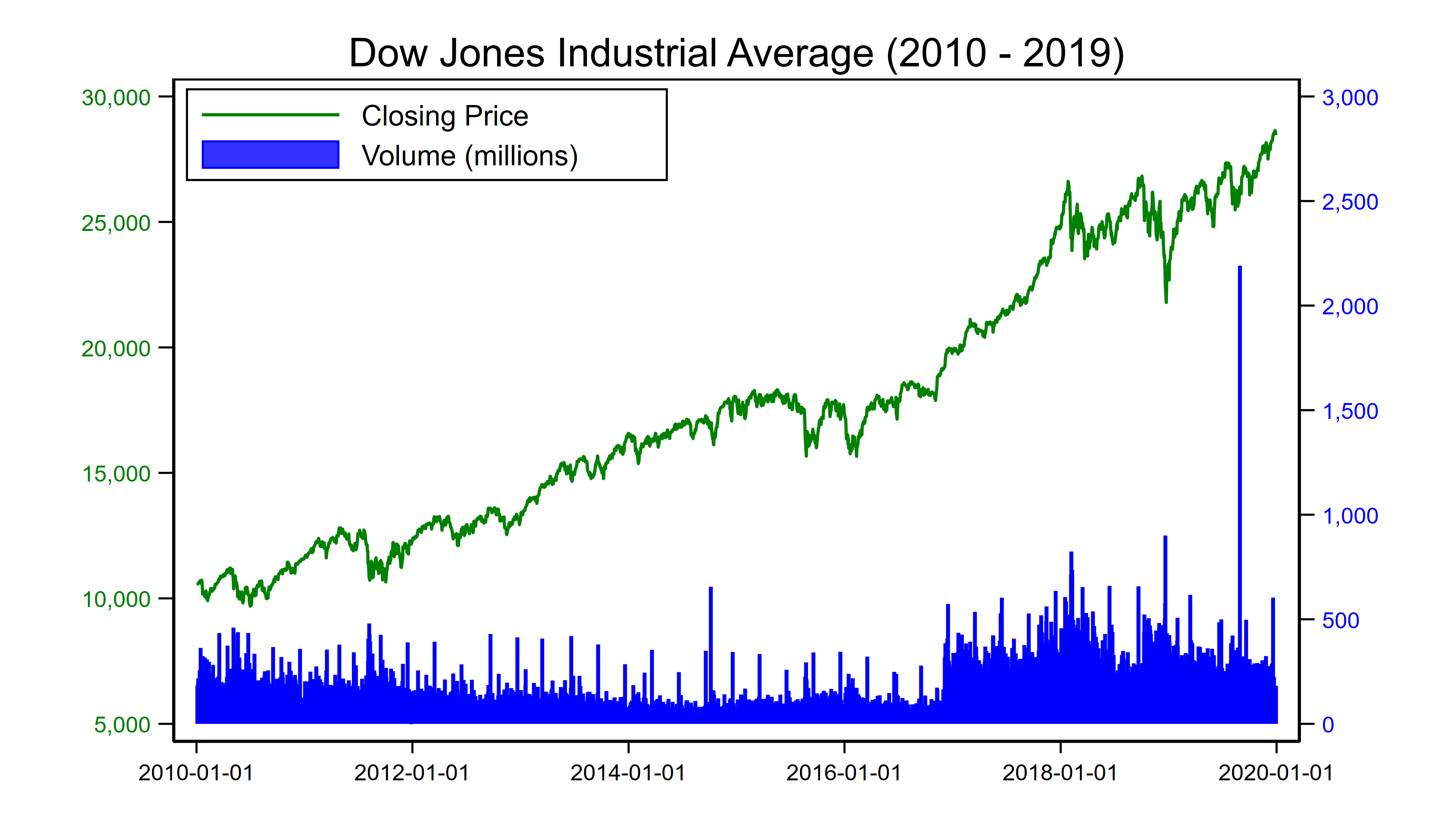
In my previous post, we learned how to use the Stata Function Interface (SFI) module to copy data from Stata to Python. In this post, I will show you how to use the SFI module to copy data from Python to Stata. We will be using the yfinance module to download financial data from the Yahoo! finance website. You can install this module in your Python environment by typing pip install yfinance. Our goal is to use Python to download historical data for the Dow Jones Industrial Average (DJIA) and use Stata to create the following graph.
If you are not familiar with Python, it may be helpful to read the first four posts in my Stata/Python Integration series before you read further.
- Setting up Stata to use Python
- Three ways to use Python in Stata
- How to install Python packages
- How to use Python packages
Using the yfinance module to download Yahoo! finance data
Let’s begin by importing the yfinance module using the alias pd. Then, we will use the download() method to download data for the DJIA from the Yahoo! finance website. The download() method accepts three arguments. The first argument is the stock symbol for the DJIA. The second argument is the start date for the stock data, and the third argument is the end date.
python:
import yfinance as yf
dowjones = yf.download("^DJI", start="2010-01-01", end="2019-12-31")
dowjones
end
The download() method returns a Pandas data frame with 2,515 rows and 6 columns indexed by date.
. python:
----------------------------------------------- python (type end to exit) ------
>>> import yfinance as yf
>>> dowjones = yf.download("^DJI", start="2010-01-01", end="2019-12-31")
[*********************100%***********************]  1 of 1 completed
>>> dowjones
                    Open          High  ...     Adj Close     Volume
Date                                    ...
2010-01-04  10430.690430  10604.969727  ...  10583.959961  179780000
2010-01-05  10584.559570  10584.559570  ...  10572.019531  188540000
2010-01-06  10564.719727  10594.990234  ...  10573.679688  186040000
2010-01-07  10571.110352  10612.370117  ...  10606.860352  217390000
2010-01-08  10606.400391  10619.400391  ...  10618.190430  172710000
...                  ...           ...  ...           ...        ...
2019-12-23  28491.779297  28582.490234  ...  28551.529297  223530000
2019-12-24  28572.570312  28576.800781  ...  28515.449219   86150000
2019-12-26  28539.460938  28624.099609  ...  28621.390625  155970000
2019-12-27  28675.339844  28701.660156  ...  28645.259766  182280000
2019-12-30  28654.759766  28664.689453  ...  28462.140625  181600000

[2515 rows x 6 columns]
>>> end
--------------------------------------------------------------------------------
We can view the details of the index by typing dowjones.index in Python. The output below shows us that the index column is named ‘Date’, which is stored as the data type datetime64[ns].
. python:
----------------------------------------------- python (type end to exit) ------
>>> dowjones.index
DatetimeIndex(['2010-01-04', '2010-01-05', '2010-01-06', '2010-01-07',
               '2010-01-08', '2010-01-11', '2010-01-12', '2010-01-13',
               '2010-01-14', '2010-01-15',
               ...
               '2019-12-16', '2019-12-17', '2019-12-18', '2019-12-19',
               '2019-12-20', '2019-12-23', '2019-12-24', '2019-12-26',
               '2019-12-27', '2019-12-30'],
              dtype='datetime64[ns]', name='Date', length=2515, freq=None)
>>> end
--------------------------------------------------------------------------------
We must convert the index to a string variable before we copy it to a Stata variable. We can use the astype() method to create a new column named dowdate that contains the index stored as a string.
. python:
----------------------------------------------- python (type end to exit) ------
>>> dowjones['dowdate'] = dowjones.index.astype(str)
>>> dowjones['dowdate']
Date
2010-01-04    2010-01-04
2010-01-05    2010-01-05
2010-01-06    2010-01-06
2010-01-07    2010-01-07
2010-01-08    2010-01-08
                 ...
2019-12-23    2019-12-23
2019-12-24    2019-12-24
2019-12-26    2019-12-26
2019-12-27    2019-12-27
2019-12-30    2019-12-30
Name: dowdate, Length: 2515, dtype: object
>>> end
--------------------------------------------------------------------------------
Use the SFI module to copy the Python data to Stata
Now, we’re ready to use the SFI module to copy the dowjones data frame to Stata. We begin by importing the Data class from the SFI module. Then, we can use the setObsTotal() method to add observations to the current Stata dataset. We must add enough observations to the Stata dataset to store all the rows of the dowjones data frame. We can count the number of rows using the
len() method.
. python:
----------------------------------------------- python (type end to exit) ------
... from sfi import Data
>>> Data.setObsTotal(len(dowjones))
>>> end
--------------------------------------------------------------------------------
Next, we will add three variables to the Stata dataset. The addVarStr() method adds a 10-character string variable named “dowdate”. The addVarDouble() method adds a double-precision variable named “dowclose”. And the addVarInt() method adds an int variable named “dowvolume”.
. python:
----------------------------------------------- python (type end to exit) ------
>>> Data.addVarStr("dowdate",10)
>>> Data.addVarDouble("dowclose")
>>> Data.addVarInt("dowvolume")
>>> end
--------------------------------------------------------------------------------
Now, we can use the store() method to copy columns from the Pandas data frame to variables in the Stata dataset. store() accepts four arguments. The first argument is the name of the Stata variable to which the Pandas column is to be copied. The second argument can be used to specify a subset of the data frame to be copied. For example, we could use the range() function to specify a range of rows to copy. I wish to copy all the observations so I have specified “None”. The third argument is the Python data that is to be copied to Stata. The fourth argument is the name of an indicator variable that specifies which rows in the Python data frame are to be copied to the Stata variable. This argument is optional. When it is not specified,
all the rows in the Python data frame are copied.
The first statement in the output below copies column dowdate from the Python data frame dowjones to the Stata variable dowdate. The second statement copies column Adj Close from the Python data frame dowjones to the Stata variable dowclose. The third statement in the output below copies column Volume from the Python data frame dowjones to the Stata variable dowvolume. Note that I have specified “None” for the second and fourth arguments because I wish to copy all the rows from the Pandas data frame.
. python:
----------------------------------------------- python (type end to exit) ------
>>> Data.store("dowdate", None, dowjones['dowdate'], None)
>>> Data.store("dowclose", None, dowjones['Adj Close'], None)
>>> Data.store("dowvolume", None, dowjones['Volume'], None)
>>> end
--------------------------------------------------------------------------------
Clean the Stata dataset
Let’s list the first five observations in our Stata dataset to check our work.
. list in 1/5, abbreviate(9)

     +-----------------------------------+
     |    dowdate   dowclose   dowvolume |
     |-----------------------------------|
  1. | 2010-01-04   10583.96     1.8e+08 |
  2. | 2010-01-05   10572.02     1.9e+08 |
  3. | 2010-01-06   10573.68     1.9e+08 |
  4. | 2010-01-07   10606.86     2.2e+08 |
  5. | 2010-01-08   10618.19     1.7e+08 |
     +-----------------------------------+
Our data look pretty good, but we have a few data management tasks to complete before we can graph the data. First, recall that dowdate is stored as a string. Let’s use Stata’s date() function to generate a new variable named date. The first argument is the string variable that is to be converted to a date. The second argument is the order of the year, month, and day in the first argument. I have specified “YMD” because the data in dowdate are stored with the year first, the month second, and the day third.
. generate date = date(dowdate,"YMD")

. list in 1/5, abbreviate(9)

     +-------------------------------------------+
     |    dowdate   dowclose   dowvolume    date |
     |-------------------------------------------|
  1. | 2010-01-04   10583.96   1.798e+08   18266 |
  2. | 2010-01-05   10572.02   1.885e+08   18267 |
  3. | 2010-01-06   10573.68   1.860e+08   18268 |
  4. | 2010-01-07   10606.86   2.174e+08   18269 |
  5. | 2010-01-08   10618.19   1.727e+08   18270 |
     +-------------------------------------------+
The data in date do not look like dates to you and me. The date() function returns the number of days since January 1, 1960. We can use format to display the data in a familiar date format.
. format %tdCCYY-NN-DD date

. list in 1/5, abbreviate(9)

     +------------------------------------------------+
     |    dowdate   dowclose   dowvolume         date |
     |------------------------------------------------|
  1. | 2010-01-04   10583.96   1.798e+08   2010-01-04 |
  2. | 2010-01-05   10572.02   1.885e+08   2010-01-05 |
  3. | 2010-01-06   10573.68   1.860e+08   2010-01-06 |
  4. | 2010-01-07   10606.86   2.174e+08   2010-01-07 |
  5. | 2010-01-08   10618.19   1.727e+08   2010-01-08 |
     +------------------------------------------------+
Next, dowvolume is displayed in scientific notation. We can again use format to display the numbers with commas in the thousands place.
. format %16.0fc dowvolume

. list in 1/5, abbreviate(9)

     +--------------------------------------------------+
     |    dowdate   dowclose     dowvolume         date |
     |--------------------------------------------------|
  1. | 2010-01-04   10583.96   179,780,000   2010-01-04 |
  2. | 2010-01-05   10572.02   188,540,000   2010-01-05 |
  3. | 2010-01-06   10573.68   186,040,000   2010-01-06 |
  4. | 2010-01-07   10606.86   217,390,000   2010-01-07 |
  5. | 2010-01-08   10618.19   172,710,000   2010-01-08 |
     +--------------------------------------------------+
It looks like dowvolume is rounded to the nearest 10,000. So let’s divide dowvolume by 1,000,000 and use format to display the data with two decimal places. Let’s also label dowvolume so that we don’t forget that the data are stored as “millions of shares”.
. replace dowvolume = dowvolume/1000000
(2,515 real changes made)

. format %10.2fc dowvolume

. label variable dowvolume "DJIA Volume (Millions of Shares)"

. list in 1/5, abbreviate(9)

     +------------------------------------------------+
     |    dowdate   dowclose   dowvolume         date |
     |------------------------------------------------|
  1. | 2010-01-04   10583.96      179.78   2010-01-04 |
  2. | 2010-01-05   10572.02      188.54   2010-01-05 |
  3. | 2010-01-06   10573.68      186.04   2010-01-06 |
  4. | 2010-01-07   10606.86      217.39   2010-01-07 |
  5. | 2010-01-08   10618.19      172.71   2010-01-08 |
     +------------------------------------------------+
Our data are formatted and ready to graph.
Graph the data
I’d like to create a graph that includes a line graph for dowclose and a bar chart for dowvolume. This is easy with graph twoway. We can use graph twoway line to create a line plot for dowclose and graph twoway bar for dowvolume. You may be familiar with many of the graphics options in the code block below. I have used title() to add a title and used xtitle(“”) and ytitle(“”) to remove the titles from the x and y axes, respectively. I have used xlabel and ylabel() to label the axes. And I have used legend() to format the legend.
The options yaxis(2) and axis(2) may be unfamiliar to you. The yaxis(2) option creates a second y axis on the right side of the graph for the bar chart. The axis(2) option in the ytitle() and ylabel() specify that those options apply to the second y axis. Note that I have plotted dowclose with a green line and labeled the left y axis with a green font to emphasize that the left axis describes the line graph. Similarly, I have I have plotted dowvolume with blue bars and labeled the right y axis with a blue font to emphasize that the right axis describes the bar graph.
twoway (line dowclose date, lcolor(green) lwidth(medium))         ///
       (bar dowvolume date, fcolor(blue) lcolor(blue) yaxis(2)),  ///
       title("Dow Jones Industrial Average (2010 - 2019)")        ///
       xtitle("") ytitle("") ytitle("", axis(2))                  ///
       xlabel(, labsize(small) angle(horizontal))                 ///
       ylabel(5000(5000)30000,                                    ///
              labsize(small) labcolor(green)                      ///
              angle(horizontal) format(%9.0fc))                   ///
       ylabel(0(500)3000,                                         ///
              labsize(small) labcolor(blue)                       ///
              angle(horizontal) axis(2))                          ///
       legend(order(1 "Closing Price" 2 "Volume (millions)")      ///
              cols(1) position(10) ring(0))
The code block above creates the following graph.
Conclusion
We did it! We used the Yahoo! finance module in Python to download data for the Dow Jones Industrial Average and import it to a Pandas data frame. We used the Stata Function Interface (SFI) module to create new variables in Stata and copy specific columns from the Pandas data frame to Stata variables. And we used graph twoway to create a graph with Stata. I have collected the examples below.
Next time, I will show you how to use the Stata Function Interface (SFI) module to copy scalars, macros, and matrices back and forth between Stata and Python.
example.do
python:
import yfinance as yf
from sfi import Data, Macro

# Use the yfinance module to download the DJIA data
dowjones = yf.download("^DJI", start="2010-01-01", end="2019-12-31")

# Display the column names
dowjones.columns
# Display the name of the index
dowjones.index.name
# Display the index data
dowjones.index
# Copy the index to a string column
dowjones['dowdate'] = dowjones.index.astype(str)
dowjones[['dowdate','Adj Close', 'Volume']]

# Set the number of observations in the Stata dataset
Data.setObsTotal(len(dowjones))  # Add observations to the current dataset

# Create the variables in the Stata dataset
Data.addVarStr("dowdate",10)
Data.addVarDouble("dowclose")
Data.addVarInt("dowvolume")

# Write the data from the Pandas data frame to the Stata variables
Data.store("dowdate", None, dowjones['dowdate'], None)
# This works too
#Data.store("dowdate", None, dowjones.index.astype(str), None)
Data.store("dowclose", None, dowjones['Adj Close'], None)
Data.store("dowvolume", None, dowjones['Volume'], None)
end

// Use the date() function to create the variable date
generate date = date(dowdate,"YMD")
format %tdCCYY-NN-DD date
label var date "Date"

// Format the variable dowclose
format %10.2f dowclose
label var dowclose "DJIA Closing Price"

// Format the variable dowvolume
replace dowvolume = dowvolume/1000000
format %10.2fc dowvolume
label var dowvolume "DJIA Volume (Millions of Shares)"

list in 1/5, abbrev(9)

// Create the graph
twoway (line dowclose date, lcolor(green) lwidth(medium))         ///
       (bar dowvolume date, fcolor(blue) lcolor(blue) yaxis(2)),  ///
       title("Dow Jones Industrial Average (2010 - 2019)")        ///
       xtitle("") ytitle("") ytitle("", axis(2))                  ///
       xlabel(, labsize(small) angle(horizontal))                 ///
       ylabel(5000(5000)30000,                                    ///
              labsize(small) labcolor(green)                      ///
              angle(horizontal) format(%9.0fc))                   ///
       ylabel(0(500)3000,                                         ///
              labsize(small) labcolor(blue)                       ///
              angle(horizontal) axis(2))                          ///
       legend(order(1 "Closing Price" 2 "Volume (millions)")      ///
              cols(1) position(10) ring(0))