Creating tables of descriptive statistics in Stata 18: The new dtable command
In Stata 17, we introduced the new collect suite of commands for creating and customizing tables and the etable command for easily creating and exporting a table of estimation results. Stata 18 offers another new command, dtable, that easily builds and exports a table of descriptive statistics, often called Table 1 in publications. Now generating tables of descriptive statistics for both categorical and continuous variables is easier than ever. It is worth mentioning that the twin commands etable and dtable are both built on the collect framework we introduced in Stata 17, so they share a lot of properties.
In this post, I’ll demonstrate how to create and export simple tables of descriptive statistics and more complex ones that display statistics by group, test for differences across groups, and more. I will also show how you can use the collect suite of commands to further customize the look of your tables and how to include tables created with dtable in complete reports.
A simple example
Before Stata 18, if we wanted to generate a table of descriptive statistics (to be included in a publication later), we might have used summarize to obtain summary statistics for continuous variables and tabulate to report the frequencies, proportions, or percentages for categorical variables. Let’s use auto.dta (1978 automobile data) to demonstrate that:
. sysuse auto, clear
(1978 automobile data)

. summarize price weight mpg

    Variable |        Obs        Mean    Std. dev.       Min        Max
-------------+---------------------------------------------------------
       price |         74    6165.257    2949.496       3291      15906
      weight |         74    3019.459    777.1936       1760       4840
         mpg |         74     21.2973    5.785503         12         41

. tabulate rep78

     Repair |
record 1978 |      Freq.     Percent        Cum.
------------+-----------------------------------
          1 |          2        2.90        2.90
          2 |          8       11.59       14.49
          3 |         30       43.48       57.97
          4 |         18       26.09       84.06
          5 |         11       15.94      100.00
------------+-----------------------------------
      Total |         69      100.00
These commands computed the statistics for us. However, manually typing all of these numbers into a nicely formatted table is tedious work, and it is not reproducible when we have new data.
In comparison, with dtable, we can type
. dtable price weight mpg i.rep78

----------------------------------------
                          Summary
----------------------------------------
N                                     74
Price              6,165.257 (2,949.496)
Weight (lbs.)        3,019.459 (777.194)
Mileage (mpg)             21.297 (5.786)
Repair record 1978
  1                             2 (2.9%)
  2                            8 (11.6%)
  3                           30 (43.5%)
  4                           18 (26.1%)
  5                           11 (15.9%)
----------------------------------------
Just as easy as that, we have built a table showing the sample size of the data, means, and standard deviations for the specified continuous variables (price, weight, and mpg), as well as frequencies and percentages for levels of the specified categorical variable (rep78).
In addition to the results for the full sample, we can request the above statistics separately for each category of a group variable such as foreign by adding the by() option:
. dtable price weight mpg i.rep78, by(foreign)

------------------------------------------------------------------------------------
                                               Car origin
                          Domestic              Foreign                Total
------------------------------------------------------------------------------------
N                             52 (70.3%)            22 (29.7%)           74 (100.0%)
Price              6,072.423 (3,097.104) 6,384.682 (2,621.915) 6,165.257 (2,949.496)
Weight (lbs.)        3,317.115 (695.364)   2,315.909 (433.003)   3,019.459 (777.194)
Mileage (mpg)             19.827 (4.743)        24.773 (6.611)        21.297 (5.786)
Repair record 1978
  1                             2 (4.2%)              0 (0.0%)              2 (2.9%)
  2                            8 (16.7%)              0 (0.0%)             8 (11.6%)
  3                           27 (56.2%)             3 (14.3%)            30 (43.5%)
  4                            9 (18.8%)             9 (42.9%)            18 (26.1%)
  5                             2 (4.2%)             9 (42.9%)            11 (15.9%)
------------------------------------------------------------------------------------
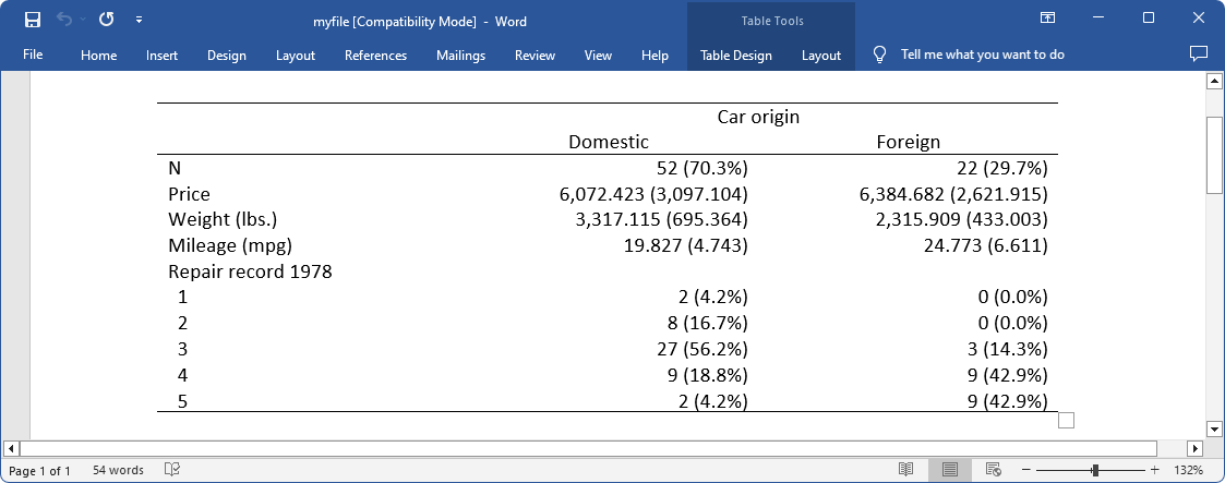
We can suppress the column for the total sample using the suboption nototal within by(). And we can export the table to a Word document, myfile.docx, using the option export():
. dtable price weight mpg i.rep78, by(foreign, nototal)
> export(myfile.docx, replace)
(output omitted)
The exported table looks like
Request customized statistics and tests
By default, dtable reports sample size for the dataset, means and standard deviations for continuous variables, and frequencies and percentages for categorical variables. But we can request other descriptive statistics such as medians and interquartile ranges. We can even specify different statistics for different variables in the same table. Before we move to a more advanced example, I want to show you the dialog box of dtable.
Go to the menu Statistics > Summaries, tables, and tests > Table of descriptive statistics to open the dialog box for dtable.
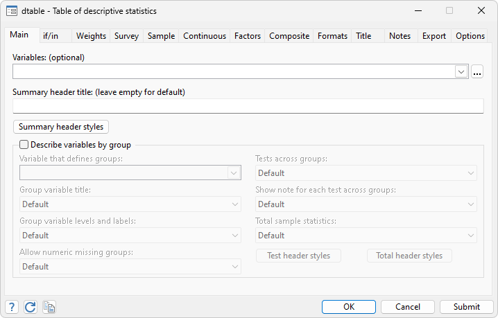
It is a good idea to browse through the tabs in the dialog box to get familiar with this command. It is a great way to explore what we can do using dtable. I want to highlight three tabs and leave the others for you to explore.
- On the Main tab, we can specify both continuous variables and categorical variables of our research interest (using the i. factor-variable notation to indicate a categorical variable). We can also specify the by variable. We can control other things like whether we want to show the test result across the by groups, whether we want to show the sample statistics, etc.
- On the Continuous tab, we can specify the continuous variables (they may or may not be specified on the Main tab), and we can request customized statistics and tests for different variables.
- The Factors tab works similarly to the Continuous tab. We can specify factor variables and choose customized statistics and tests for different variables there.
For an example, we will load the Modified Bangkok IDU Preparatory Study data provided in Zeng, Mao, and Lin (2016). We may want to try specifying customized statistics and tests for different variables instead of generating the default table. Here I used the dialog box (mainly the three tabs I mentioned above) to easily build the table, and the corresponding syntax is displayed in the output below.
. webuse idu
(Modified Bangkok IDU Preparatory Study)

. dtable, by(male, tests testnotes nototal) sample(, statistic(frequency proportion))
> continuous(age, statistics( mean min max) test(kwallis))
> continuous(ltime rtime, statistics(mean skewness kurtosis) test(poisson))
> factor(needle, statistics(fvfrequency fvproportion))
> factor(jail inject, statistics(fvfrequency) test(fisher))
note: using test kwallis across levels of male for age.
note: using test poisson across levels of male for ltime and rtime.
note: using test pearson across levels of male for needle.
note: using test fisher across levels of male for jail and inject.

----------------------------------------------------------------------------------
                                                        Male
                                           No                   Yes          Test
----------------------------------------------------------------------------------
N                                             76 0.068          1,048 0.932
Age (in years)                    28.776 18.000 46.000 31.656 17.000 52.000  0.002
Last time seronegative for HIV-1   22.129 -0.305 2.017  24.323 -0.353 2.251 <0.001
First time seropositive for HIV-1   11.951 0.951 2.285   14.428 0.749 3.024  0.020
Shared needles
  No                                          43 0.566            679 0.648  0.149
  Yes                                         33 0.434            369 0.352
Imprisoned at recruitment
  No                                                21                  351  0.315
  Yes                                               55                  697
Injected drugs before recruitment
  No                                                47                  659  0.902
  Yes                                               29                  389
----------------------------------------------------------------------------------
In this table, we request that the following descriptive statistics be reported: 1) the mean, minimum, and maximum values for the variable age; 2) the mean, skewness, and kurtosis for the variables ltime and rtime; 3) frequencies and proportions for the variable needle; and 4) just frequencies for the variables jail and inject. The statistics are reported separately for each level of the group variable male. And we also show the sample size and proportion for each group.
You may notice we have added a column of customized tests to compare the variables across the groups. The tests can only be included when there is a by variable specified. The specific tests we choose for different variables are mentioned clearly in the notes (before the table) because we have specified the by() suboption testnotes.
The available test types for continuous variables are the following:
| regress | main effects test from a linear regression (t test) | |
| poisson | main effects test from a Poisson regression | |
| lnormal | main effects test from a log-normal regression | |
| kwallis | Kruskal–Wallis rank test |
| pearson | Pearson's chi-squared test | |
| fisher | Fisher's exact test | |
| lrchi2 | likelihood-ratio chi-squared test | |
| gamma | Goodman and Kruskal's gamma | |
| kendall | Kendall's \(\tau\) | |
| cramer | Cramér's V | |
| svylr | survey-adjusted likelihood-ratio test | |
| svywald | survey-adjusted Wald test | |
| svyllwald | survey-adjusted log-linear Wald test | |
| none | suppress the test |
| Suffix | File format | Output format |
| docx | as(docx) | Microsoft Word |
| html | as(html) | HTML 5 with CSS |
| as(pdf) | ||
| xlsx | as(xlsx) | Microsoft Excel 2007/2010 or newer |
| xls | as(xls) | Microsoft Excel 1997/2003 |
| tex | as(latex) | LaTeX |
| smcl | as(smcl) | SMCL |
| txt | as(txt) | Plain text |
| markdown | as(markdown) | Markdown |
| md | as(markdown) | Markdown |
Further customize the table using collect
The table above looks nice. But I will demonstrate how to make some additional changes not directly available with dtable. Because dtable is implemented using collect, we can use the collect suite of commands to further manage tables that were created using dtable and to edit them in various ways. By the way, collect commands require a little effort at the beginning to become familiar with all the tools, but I believe you will master the skills and love to use this suite of commands to create any tables you need after a little bit of practice. If you would like to learn about collect, you can view our reference manual of Customizable Tables and Collected Results.
Regarding the further changes, I want to 1) hide the variable name male in the table header and change the group labels No and Yes to Female and Male, respectively, 2) add horizontal lines between continuous variables and categorical variables and also between different categorical variables, 3) bold the p-values for the tests and highlight the test column with a light-yellow shade, and 4) add customized notes to the table showing the test types for different variables. Let's use the following collect commands to make these changes:
. collect style header male, title(hide)

. collect label levels male 0 "Female", modify

. collect label levels male 1 "Male", modify

. collect style cell var[rtime 1.needle 1.jail], border( bottom, width(1))

. collect style cell male[_dtable_test], shading( background(lightyellow)) font(, bold)

. collect notes "Kruskal–Wallis rank test performed for age."

. collect notes "Poisson regression main effects test performed for ltime and rtime."

. collect notes "Pearson's chi-squared test performed for needle."

. collect notes "Fisher's exact test performed for jail and inject."

. collect layout
Please note the Stata Results window can show some of these changes, but it cannot show modifications such as the shading color. We can open the Tables builder and confirm there that we have the exact table style that we wanted. We can open the Tables builder from the menu by clicking on Statistics > Summaries, tables, and tests > Tables and collections > Build and style table.
We can see how the table looks right now in the preview window in the Tables builder.
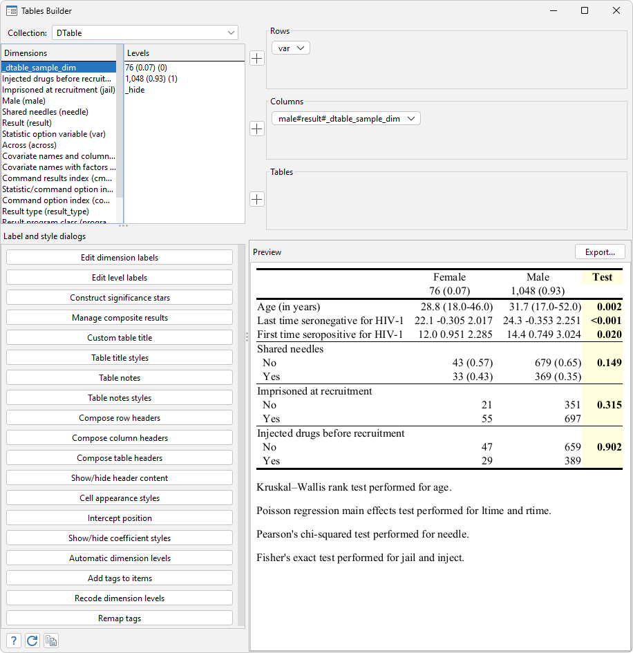
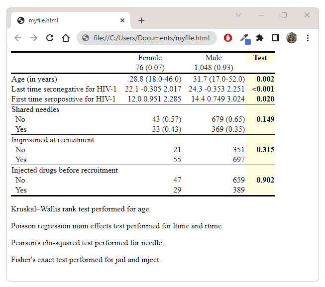
When we export the table to other documents, the exported table will look the same as what is shown here. Now let us export the table to an .html file.
. collect export myfile.html, replace
Here is our resulting document:
Generate a full report including the table
Because dtable creates tables of descriptive statistics, and this type of table is usually included as Table 1 in technical manuscripts, you may want to insert the table obtained with dtable into a larger document instead of solely exporting the table as a document. If that is the case, you can use putdocx collect, putpdf collect, or putexcel ul_cell = collect to export the table if you are creating a document using, respectively, putdocx, putpdf, or putexcel. In this way, the table can be put anywhere in the document along with other content. Here is an example of using putdocx to create a document including the above table:
webuse idu, clear
putdocx clear
putdocx begin
// Add a title
putdocx paragraph, style(Title)
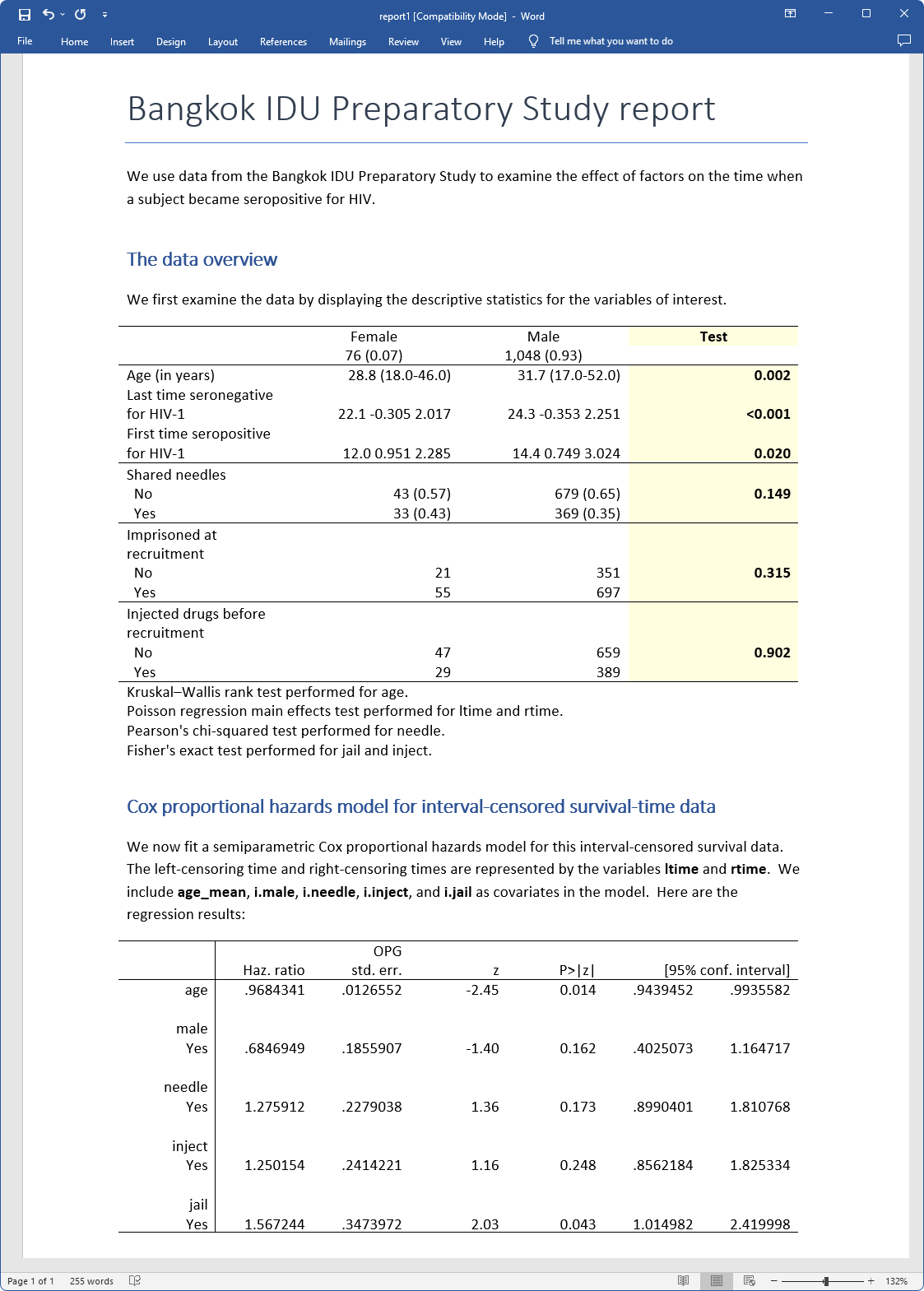
putdocx text ("Bangkok IDU Preparatory Study report")
putdocx textblock begin
We use data from the Bangkok IDU Preparatory Study to examine
the effect of factors on the time when a subject became
seropositive for HIV.
putdocx textblock end
// Add a heading
putdocx paragraph, style(Heading1)
putdocx text ("The data overview")
putdocx textblock begin
We first examine the data by displaying the descriptive
statistics for the variables of interest.
putdocx textblock end
dtable, by(male, tests testnotes nototal) ///
sample(, statistic(frequency proportion) ///
place(seplabels) ) continuous(age, statistics(mean minmax) test(kwallis)) ///
continuous(ltime rtime, statistics(mean skewness kurtosis) test(poisson)) ///
factor(needle, statistics(fvfrequency fvproportion)) ///
factor(jail inject, statistics(fvfrequency) test(fisher)) ///
define(minmax = min max, delimiter(-)) nformat(%9.1f mean minmax) ///
sformat("(%s)" fvproportion minmax proportion) ///
nformat(%9.2f proportion fvproportion)
collect style header male, title(hide)
collect label levels male 0 "Female", modify
collect label levels male 1 "Male", modify
collect style cell var[rtime 1.needle 1.jail], border( bottom, width(1))
collect style cell male[_dtable_test], shading( background(lightyellow)) ///
font(, bold)
collect notes "Kruskal–Wallis rank test performed for age."
collect notes "Poisson regression main effects test performed for ltime and rtime."
collect notes "Pearson's chi-squared test performed for needle."
collect notes "Fisher's exact test performed for jail and inject."
putdocx collect
putdocx paragraph, style(Heading1)
putdocx text ("Cox proportional hazards model for interval-censored survival-time data")
putdocx textblock begin
We now fit a semiparametric Cox proportional hazards model for this
interval-censored survival data. The left-censoring time and
right-censoring times are represented by the variables
<<dd_docx_display bold: "ltime">> and
<<dd_docx_display bold: "rtime">>. We include
<<dd_docx_display bold: "age_mean">>, <<dd_docx_display bold: "i.male">>,
<<dd_docx_display bold: "i.needle">>, <<dd_docx_display bold: "i.inject">>,
and <<dd_docx_display bold: "i.jail">> as covariates in the model.
Here are the regression results:
putdocx textblock end
stintcox age i.male i.needle i.inject i.jail, interval(ltime rtime)
putdocx table results = etable
putdocx save report1, replace
Using the above code, we create the file report1.docx, which looks like
This report is also reproducible. Rerun your commands at any time and re-create your report. You can see https://www.stata.com/features/overview/truly-reproducible-reporting/ for more information regarding reproducible reports.
Summary
In this blog post, I have shown you some of the features and fun things you can do using dtable in Stata 18. It has so many features that I cannot show them all in one post. Now you may be ready to open your Stata and try dtable yourself. I hope I have provided you with some useful demonstrations, and that may give you a good start.
To read more about dtable, please visit
You can also watch the following video tutorial on our YouTube channel:
Reference
Zeng, D., L. Mao, and D. Lin. 2016. Maximum likelihood estimation for semiparametric transformation models with interval-censored data. Biometrika 103: 253–271. https://doi.org/10.1093/biomet/asw013