Introduction
Three months ago, I wrote about a new command, twitter2stata, that imports data from Twitter’s REST API into Stata. Today, I will show you the tools we used to develop this command. Writing this command from scratch solely in Mata or ado-code would have taken several months. Fortunately, we can significantly speed up our development using an existing Java library (Twitter4J) and Stata’s Java plugins. In this post, I will discuss the basic steps of how to leverage a Java library and the Stata Java API.
Java is the most popular programming language in the world, so there are many libraries to support your development. A quick Google search should tell you if a Java library exists for what you are trying to do; this is how we found the library Twitter4J. For the rest of this blog entry, a basic understanding of programming in Java is helpful, but not necessary. Read more…
We announced Stata 15 today. It’s a big deal because this is Stata’s biggest release ever.
I posted to Statalist this morning and listed sixteen of the most important new features. Here on the blog I will say more about them, and you can learn even more by visiting our website and seeing the Stata 15 features page.
I go into depth below on the sixteen highlighted features. They are (click to jump)
Read more…
In my last post, I demonstrated how to use putexcel to recreate common Stata output in Microsoft Excel. Today I want to show you how to create custom reports for arbitrary variables. I am going to create tables that combine cell counts with row percentages, and means with standard deviations. But you could modify the examples below to include column percentages, percentiles, standard errors, confidence intervals or any statistic. I am also going to pass the variable names into my programs using local macros. This will allow me to create the same report for arbitrary variables by simply assigning new variable names to the macros. You could extend this idea by creating a do-file for each report and passing the variable names into the do-files. This is another important step toward our goal of automating the creation of reports in Excel.
Today’s blog post is Read more…
In my last post, I showed how to use putexcel to write simple expressions to Microsoft Excel and format the resulting text and cells. Today, I want to show you how to write more complex expressions such as macros, graphs, and matrices. I will even show you how to write formulas to Excel to create calculated cells. These are important steps toward our goal of automating the creation of reports in Excel.
Before we begin the examples, Read more…
For a long time, I have wanted to type a Stata command like this,
. ExcelTable race, cont(age height weight) cat(sex diabetes)
The Excel table table.xlsx was created successfully
and get an Excel table that looks like this:
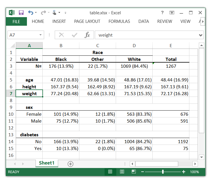
So I wrote a program called ExcelTable for my own use Read more…
estat commands display statistics after estimation. Many of these statistics are diagnostics or tests used to evaluate model specification. Some statistics are available after all estimation commands; others are command specific.
I illustrate how estat commands work and then show how to write a command-specific estat command for the mypoisson command that I have been developing.
This is the 28th post in the series Programming an estimation command in Stata. I recommend that you start at the beginning. See Programming an estimation command in Stata: A map to posted entries for a map to all the posts in this series. Read more…
\(
\newcommand{\xb}{{\bf x}}
\newcommand{\gb}{{\bf g}}
\newcommand{\Hb}{{\bf H}}
\newcommand{\Gb}{{\bf G}}
\newcommand{\Eb}{{\bf E}}
\newcommand{\betab}{\boldsymbol{\beta}}
\)I write ado-commands that estimate the parameters of an exponential conditional mean (ECM) model and a probit conditional mean (PCM) model by nonlinear least squares, using the methods that I discussed in the post Programming an estimation command in Stata: Nonlinear least-squares estimators. These commands will either share lots of code or repeat lots of code, because they are so similar. It is almost always better to share code than to repeat code. Shared code only needs to be changed in one place to add a feature or to fix a problem; repeated code must be changed everywhere. I introduce Mata libraries to share Mata functions across ado-commands, and I introduce wrapper commands to share ado-code.
This is the 27th post in the series Programming an estimation command in Stata. I recommend that you start at the beginning. See Programming an estimation command in Stata: A map to posted entries for a map to all the posts in this series.
Ado-commands for ECM and PCM models
I now convert the examples of Read more…
\(\newcommand{\xb}{{\bf x}}
\newcommand{\gb}{{\bf g}}
\newcommand{\Hb}{{\bf H}}
\newcommand{\Gb}{{\bf G}}
\newcommand{\Eb}{{\bf E}}
\newcommand{\betab}{\boldsymbol{\beta}}\)I want to write ado-commands to estimate the parameters of an exponential conditional mean (ECM) model and probit conditional mean (PCM) model by nonlinear least squares (NLS). Before I can write these commands, I need to show how to trick optimize() into performing the Gauss–Newton algorithm and apply this trick to these two problems.
This is the 26th post in the series Programming an estimation command in Stata. I recommend that you start at the beginning. See Programming an estimation command in Stata: A map to posted entries for a map to all the posts in this series.
Gauss–Newton algorithm
Gauss–Newton algorithms frequently perform better than Read more…
\(\newcommand{\xb}{{\bf x}}
\newcommand{\betab}{\boldsymbol{\beta}}\)Before you use or distribute your estimation command, you should verify that it produces correct results and write a do-file that certifies that it does so. I discuss the processes of verifying and certifying an estimation command, and I present some techniques for writing a do-file that certifies mypoisson5, which I discussed in previous posts.
This is the twenty-fifth post in the series Programming an estimation command in Stata. I recommend that you start at the beginning. See Programming an estimation command in Stata: A map to posted entries for a map to all the posts in this series.
Verification versus certification
Verification is the process of establishing Read more…
I make predict work after mypoisson5 by writing an ado-command that computes the predictions and by having mypoisson5 store the name of this new ado-command in e(predict). The ado-command that computes predictions using the parameter estimates computed by ado-command mytest should be named mytest_p, by convention. In the next section, I discuss mypoisson5_p, which computes predictions after mypoisson5. In section Storing the name of the prediction command in e(predict), I show that storing the name mypoisson5_p in e(predict) requires only a one-line change to mypoisson4.ado, which I discussed in Programming an estimation command in Stata: Adding analytical derivatives to a poisson command using Mata.
This is the twenty-fourth post in the Read more…