Distributing a Stata command that implements a statistical method will get that method used by lots of people. They will thank you. And, they will cite you!
This post is the first in the series #StataProgramming about programing an estimation command in Stata that uses Mata to do the numerical work. In the process of showing you how to program an estimation command in Stata, I will discuss do-file programming, ado-file programming, and Mata programming. When the series ends, you will be able to write Stata commands.
Stata users like its predictable syntax and its estimation-postestimation structure that facilitates hypothesis testing, specification tests, and parameter interpretation. To help you write Stata commands that people want to use, I illustrate how Stata syntax is predictable and give an overview of the estimation-postestimation structure that you will want to emulate in your programs. Read more…
\(\newcommand{\epsilonb}{\boldsymbol{\epsilon}}
\newcommand{\ebi}{\boldsymbol{\epsilon}_i}
\newcommand{\Sigmab}{\boldsymbol{\Sigma}}
\newcommand{\Omegab}{\boldsymbol{\Omega}}
\newcommand{\Lambdab}{\boldsymbol{\Lambda}}
\newcommand{\betab}{\boldsymbol{\beta}}
\newcommand{\gammab}{\boldsymbol{\gamma}}
\newcommand{\Gammab}{\boldsymbol{\Gamma}}
\newcommand{\deltab}{\boldsymbol{\delta}}
\newcommand{\xib}{\boldsymbol{\xi}}
\newcommand{\iotab}{\boldsymbol{\iota}}
\newcommand{\xb}{{\bf x}}
\newcommand{\xbit}{{\bf x}_{it}}
\newcommand{\xbi}{{\bf x}_{i}}
\newcommand{\zb}{{\bf z}}
\newcommand{\zbi}{{\bf z}_i}
\newcommand{\wb}{{\bf w}}
\newcommand{\yb}{{\bf y}}
\newcommand{\ub}{{\bf u}}
\newcommand{\Gb}{{\bf G}}
\newcommand{\Hb}{{\bf H}}
\newcommand{\thetab}{\boldsymbol{\theta}}
\newcommand{\XBI}{{\bf x}_{i1},\ldots,{\bf x}_{iT}}
\newcommand{\Sb}{{\bf S}} \newcommand{\Xb}{{\bf X}}
\newcommand{\Xtb}{\tilde{\bf X}}
\newcommand{\Wb}{{\bf W}}
\newcommand{\Ab}{{\bf A}}
\newcommand{\Bb}{{\bf B}}
\newcommand{\Zb}{{\bf Z}}
\newcommand{\Eb}{{\bf E}}\) This post was written jointly with Joerg Luedicke, Senior Social Scientist and Statistician, StataCorp.
Overview
We provide an introduction to parameter estimation by maximum likelihood and method of moments using mlexp and gmm, respectively (see [R] mlexp and [R] gmm). We include some background about these estimation techniques; see Pawitan (2001, Casella and Berger (2002), Cameron and Trivedi (2005), and Wooldridge (2010) for more details.
Maximum likelihood (ML) estimation finds the parameter values that make the observed data most probable. The parameters maximize the log of the likelihood function that specifies the probability of observing a particular set of data given a model.
Method of moments (MM) estimators specify population moment conditions and find the parameters that solve the equivalent sample moment conditions. MM estimators usually place fewer restrictions on the model than ML estimators, which implies that MM estimators are less efficient but more robust than ML estimators. Read more…
Overview
In this post, I show how to use Monte Carlo simulations to compare the efficiency of different estimators. I also illustrate what we mean by efficiency when discussing statistical estimators.
I wrote this post to continue a dialog with my friend who doubted the usefulness of the sample average as an estimator for the mean when the data-generating process (DGP) is a \(\chi^2\) distribution with \(1\) degree of freedom, denoted by a \(\chi^2(1)\) distribution. The sample average is a fine estimator, even though it is not the most efficient estimator for the mean. (Some researchers prefer to estimate the median instead of the mean for DGPs that generate outliers. I will address the trade-offs between these parameters in a future post. For now, I want to stick to estimating the mean.)
In this post, I also want to illustrate that Monte Carlo simulations can help explain abstract statistical concepts. I show how to use a Monte Carlo simulation to illustrate the meaning of an abstract statistical concept. (If you are new to Monte Carlo simulations in Stata, you might want to see Monte Carlo simulations using Stata.) Read more…
Overview
In this post, I show how to use mlexp to estimate the degree of freedom parameter of a chi-squared distribution by maximum likelihood (ML). One example is unconditional, and another example models the parameter as a function of covariates. I also show how to generate data from chi-squared distributions and I illustrate how to use simulation methods to understand an estimation technique. Read more…
Overview
A Monte Carlo simulation (MCS) of an estimator approximates the sampling distribution of an estimator by simulation methods for a particular data-generating process (DGP) and sample size. I use an MCS to learn how well estimation techniques perform for specific DGPs. In this post, I show how to perform an MCS study of an estimator in Stata and how to interpret the results.
Large-sample theory tells us that the sample average is a good estimator for the mean when the true DGP is a random sample from a \(\chi^2\) distribution with 1 degree of freedom, denoted by \(\chi^2(1)\). But a friend of mine claims this estimator will not work well for this DGP because the \(\chi^2(1)\) distribution will produce outliers. In this post, I use an MCS to see if the large-sample theory works well for this DGP in a sample of 500 observations. Read more…
This post was written jointly with David Drukker, Director of Econometrics, StataCorp.
In our last post, we introduced the concept of treatment effects and demonstrated four of the treatment-effects estimators that were introduced in Stata 13. Today, we will talk about two more treatment-effects estimators that use matching. Read more…
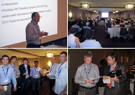
We are happy to report another successful Stata Conference is in the books! Attendees had the opportunity to network, learn, and share their experiences with the Stata community.
We’d like to thank the organizers and everyone who participated in making this year’s conference one of the best yet. Here’s what attendees had to say on social media.
As the conference approached, the countdown began. Read more…
New to Stata 14 is a suite of commands to fit item response theory (IRT) models. IRT models are used to analyze the relationship between the latent trait of interest and the items intended to measure the trait. Stata’s irt commands provide easy access to some of the commonly used IRT models for binary and polytomous responses, and irtgraph commands can be used to plot item characteristic functions and information functions.
To learn more about Stata’s IRT features, I refer you to the [IRT] manual; here I want to go beyond the manual and show you a couple of examples of what you can do with a little bit of Stata code. Read more…
This post was written jointly with David Drukker, Director of Econometrics, StataCorp.
The topic for today is the treatment-effects features in Stata.
Treatment-effects estimators estimate the causal effect of a treatment on an outcome based on observational data.
In today’s posting, we will discuss four treatment-effects estimators:
- RA: Regression adjustment
- IPW: Inverse probability weighting
- IPWRA: Inverse probability weighting with regression adjustment
- AIPW: Augmented inverse probability weighting
We’ll save the matching estimators for part 2.
We should note that nothing about treatment-effects estimators magically extracts causal relationships. As with any regression analysis of observational data, the causal interpretation must be based on a reasonable underlying scientific rationale. Read more…
The Stata Conference connects you with the best and the brightest of the Stata community, offering a variety of presentations from Stata users and StataCorp experts. This year’s conference will be held July 30-31, 2015, in Columbus, Ohio, and is open to all Stata users wishing to attend.

With the conference just around the corner, we want to suggest a few things to do that will help maximize your experience. Read more…
