Initial thoughts

Estimating causal relationships from data is one of the fundamental endeavors of researchers, but causality is elusive. In the presence of omitted confounders, endogeneity, omitted variables, or a misspecified model, estimates of predicted values and effects of interest are inconsistent; causality is obscured.

A controlled experiment to estimate causal relations is an alternative. Yet conducting a controlled experiment may be infeasible. Policy makers cannot randomize taxation, for example. In the absence of experimental data, an option is to use instrumental variables or a control function approach.

Stata has many built-in estimators to implement these potential solutions and tools to construct estimators for situations that are not covered by built-in estimators. Below I illustrate both possibilities for a linear model and, in a later post, will talk about nonlinear models. Read more…

In my last post, I showed how to use putexcel to write simple expressions to Microsoft Excel and format the resulting text and cells. Today, I want to show you how to write more complex expressions such as macros, graphs, and matrices. I will even show you how to write formulas to Excel to create calculated cells. These are important steps toward our goal of automating the creation of reports in Excel.

Before we begin the examples, Read more…

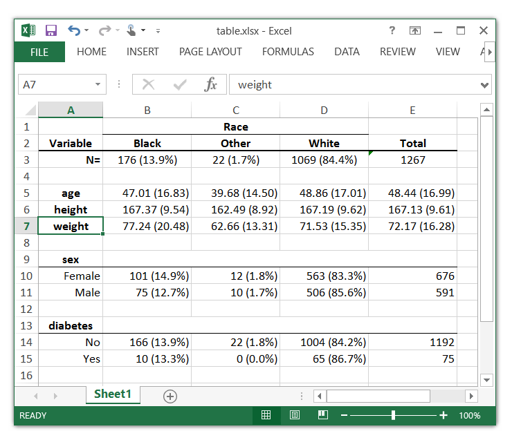
For a long time, I have wanted to type a Stata command like this,

. ExcelTable race, cont(age height weight) cat(sex diabetes)
The Excel table table.xlsx was created successfully

and get an Excel table that looks like this:

So I wrote a program called ExcelTable for my own use Read more…

Truncation and censoring are two distinct phenomena that cause our samples to be incomplete. These phenomena arise in medical sciences, engineering, social sciences, and other research fields. If we ignore truncation or censoring when analyzing our data, our estimates of population parameters will be inconsistent.

Truncation or censoring happens during the sampling process. Let’s begin by defining left-truncation and left-censoring:

Our data are left-truncated when individuals below a threshold are not present in the sample. For example, if we want to study the size of certain fish based on the specimens captured with a net, fish smaller than the net grid won’t be present in our sample.

Our data are left-censored at \(\kappa\) if every individual with a value below \(\kappa\) is present in the sample, but the actual value is unknown. This happens, for example, when we have a measuring instrument that cannot detect values below a certain level.

We will focus our discussion on left-truncation and left-censoring, but the concepts we will discuss generalize to all types of censoring and truncation—right, left, and interval.

When performing estimations with truncated or censored data, we need to use tools that account for that type of incomplete data. For truncated linear regression, we can use the truncreg command, and for censored linear regression, we can use the intreg or tobit command.

In this blog post, we will analyze the characteristics of truncated and censored data and discuss using truncreg and tobit to account for the incomplete data. Read more…

In this blog post, I’d like to give you a relatively nontechnical introduction to Markov chain Monte Carlo, often shortened to “MCMC”. MCMC is frequently used for fitting Bayesian statistical models. There are different variations of MCMC, and I’m going to focus on the Metropolis–Hastings (M–H) algorithm. In the interest of brevity, I’m going to omit some details, and I strongly encourage you to read the [BAYES] manual before using MCMC in practice.

Let’s continue with the coin toss example from my previous post Introduction to Bayesian statistics, part 1: The basic concepts. We are interested in the posterior distribution of the parameter \(\theta\), which is the probability that a coin toss results in “heads”. Our prior distribution is a flat, uninformative beta distribution with parameters 1 and 1. And we will use a binomial likelihood function to quantify the data from our experiment, which resulted in 4 heads out of 10 tosses. Read more…

In this blog post, I’d like to give you a relatively nontechnical introduction to Bayesian statistics. The Bayesian approach to statistics has become increasingly popular, and you can fit Bayesian models using the bayesmh command in Stata. This blog entry will provide a brief introduction to the concepts and jargon of Bayesian statistics and the bayesmh syntax. In my next post, I will introduce the basics of Markov chain Monte Carlo (MCMC) using the Metropolis–Hastings algorithm. Read more…

\(\def\bfA{{\bf A}}
\def\bfB{{\bf }}
\def\bfC{{\bf C}}\)Introduction

In this blog post, I describe Stata’s capabilities for estimating and analyzing vector autoregression (VAR) models with long-run restrictions by replicating some of the results of Blanchard and Quah (1989). Read more…

estat commands display statistics after estimation. Many of these statistics are diagnostics or tests used to evaluate model specification. Some statistics are available after all estimation commands; others are command specific.

I illustrate how estat commands work and then show how to write a command-specific estat command for the mypoisson command that I have been developing.

This is the 28th post in the series Programming an estimation command in Stata. I recommend that you start at the beginning. See Programming an estimation command in Stata: A map to posted entries for a map to all the posts in this series. Read more…

Have you seen the latest issue of the Stata News? It has a new format that we think you will love. And, I want to make sure that you are not missing out on the articles discussing what our developers and users are doing with Stata.

We have a new section, User’s corner, that highlights interesting, useful, and fun user contributions. In this issue, you will see how Belén Chavez uses Stata to analyze her Fitbit® data.

We kept your favorite sections, including Spotlight articles written by Stata developers. In this issue, Enrique Pinzón demonstrates Estimating, graphing, and interpreting interactions using margins.

If you haven’t been reading the Stata News, you may want to browse previous Spotlight articles on topics such as endogenous treatment effects, item response theory (IRT), and Bayesian analysis. You can find all the previous Spotlight articles here.

We discuss estimating population-averaged parameters when some of the data are missing. In particular, we show how to use gmm to estimate population-averaged parameters for a probit model when the process that causes some of the data to be missing is a function of observable covariates and a random process that is independent of the outcome. This type of missing data is known as missing at random, selection on observables, and exogenous sample selection.

This is a follow-up to an earlier post where we estimated the parameters of a probit model under endogenous sample selection (http://blog.stata.com/2015/11/05/using-mlexp-to-estimate-endogenous-treatment-effects-in-a-probit-model/). In endogenous sample selection, the random process that affects which observations are missing is correlated with an unobservable random process that affects the outcome. Read more…