In my last two posts, I showed you how to calculate power for a t test using Monte Carlo simulations and how to integrate your simulations into Stata’s power command. In today’s post, I’m going to show you how to do these tasks for linear and logistic regression models. The strategy and overall structure of the programs for linear and logistic regression are similar to the t test examples. The parts that will change are the simulation of the data and the models used to test the null hypothesis. Read more…

In my last post, I showed you how to calculate power for a t test using Monte Carlo simulations. In this post, I will show you how to integrate your simulations into Stata’s power command so that you can easily create custom tables and graphs for a range of parameter values. Read more…

Power and sample-size calculations are an important part of planning a scientific study. You can use Stata’s power commands to calculate power and sample-size requirements for dozens of commonly used statistical tests. But there are no simple formulas for more complex models such as multilevel/longitudinal models and structural equation models (SEMs). Monte Carlo simulations are one way to calculate power and sample-size requirements for complex models, and Stata provides all the tools you need to do this. You can even integrate your simulations into Stata’s power commands so that you can easily create custom tables and graphs for a range of parameter values. Read more…

In his blog post, Enrique Pinzon discussed how to perform regression when we don’t want to make any assumptions about functional form—use the npregress command. He concluded by asking and answering a few questions about the results using the margins and marginsplot commands.

Recently, I have been thinking about all the different types of questions that we could answer using margins after nonparametric regression, or really after any type of regression. margins and marginsplot are powerful tools for exploring the results of a model and drawing many kinds of inferences. In this post, I will show you how to ask and answer very specific questions and how to explore the entire response surface based on the results of your nonparametric regression.
Read more…

What are DSGE models?

Dynamic stochastic general equilibrium (DSGE) models are used by macroeconomists to model multiple time series. A DSGE model is based on economic theory. A theory will have equations for how individuals or sectors in the economy behave and how the sectors interact. What emerges is a system of equations whose parameters can be linked back to the decisions of economic actors. In many economic theories, individuals take actions based partly on the values they expect variables to take in the future, not just on the values those variables take in the current period. The strength of DSGE models is that they incorporate these expectations explicitly, unlike other models of multiple time series.

DSGE models are often used in the analysis of shocks or counterfactuals. A researcher might subject the model economy to an unexpected change in policy or the environment and see how variables respond. For example, what is the effect of an unexpected rise in interest rates on output? Or a researcher might compare the responses of economic variables with different policy regimes. For example, a model might be used to compare outcomes under a high-tax versus a low-tax regime. A researcher would explore the behavior of the model under different settings for tax rate parameters, holding other parameters constant.

In this post, I show you how to estimate the parameters of a DSGE model, how to create and interpret an impulse response, and how to compare the impulse response estimated from the data with an impulse response generated by a counterfactual policy regime. Read more…

Ermistatas is our most popular t-shirt these days. See it and you will understand why.

We call the character Ermistatas and he is thinking—Ermistatas cogitatu. Notice the electricity bolts being emitted and received by his three antennae.

The shirt is popular even among those who do not use Stata and it’s leading them to ask questions. “Who or what is Ermistatas and why is he, she, or it deserving of a t-shirt?”. Then they add, “And why three and not the usual two antennae?”

Ermistatas is the creation of our arts-and-graphics department to represent Stata 15’s new commands for fitting Extended Regression Models—a term we coined. We call it ERMs for short. The new commands are Read more…

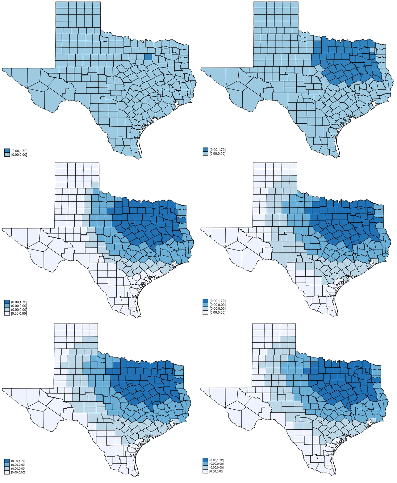
This post shows how to create animated graphics that illustrate the spatial spillover effects generated by a spatial autoregressive (SAR) model. After reading this post, you could create an animated graph like the following.

This post is organized as follows. First, I estimate the parameters of a SAR model. Second, I show why a SAR model can produce spatial spillover effects. Finally, I show how to create an animated graph that illustrates the spatial spillover effects. Read more…

You have a model that is nonlinear in the parameters. Perhaps it is a model of tree growth and therefore asymptotes to a maximum value. Perhaps it is a model of serum concentrations of a drug that rise rapidly to a peak concentration and then decay exponentially. Easy enough, use nonlinear regression ([R] nl) to fit your model. But … what if you have repeated measures for each tree or repeated blood serum levels for each patient? You might want to account for the correlation within tree or patient. You might even believe that each tree has its own asymptotic growth. You need nonlinear mixed-effects models—also called nonlinear hierarchical models or nonlinear multilevel models. Read more…

Introduction

Stata 15 provides a convenient and elegant way of fitting Bayesian regression models by simply prefixing the estimation command with bayes. You can choose from 45 supported estimation commands. All of Stata’s existing Bayesian features are supported by the new bayes prefix. You can use default priors for model parameters or select from many prior distributions. I will demonstrate the use of the bayes prefix for fitting a Bayesian logistic regression model and explore the use of Cauchy priors (available as of the update on July 20, 2017) for regression coefficients. Read more…

Introduction

Dynamic stochastic general equilibrium (DSGE) models are used in macroeconomics to model the joint behavior of aggregate time series like inflation, interest rates, and unemployment. They are used to analyze policy, for example, to answer the question, “What is the effect of a surprise rise in interest rates on inflation and output?” To answer that question we need a model of the relationship among interest rates, inflation, and output. DSGE models are distinguished from other models of multiple time series by their close connection to economic theory. Macroeconomic theories consist of systems of equations that are derived from models of the decisions of households, firms, policymakers, and other agents. These equations form the DSGE model. Because the DSGE model is derived from theory, its parameters can be interpreted directly in terms of the theory.

In this post, I build a small DSGE model that is similar to models used for monetary policy analysis. I show how to estimate the parameters of this model using the new dsge command in Stata 15. I then shock the model with a contraction in monetary policy and graph the response of model variables to the shock. Read more…