For a long time, I have wanted to type a Stata command like this,

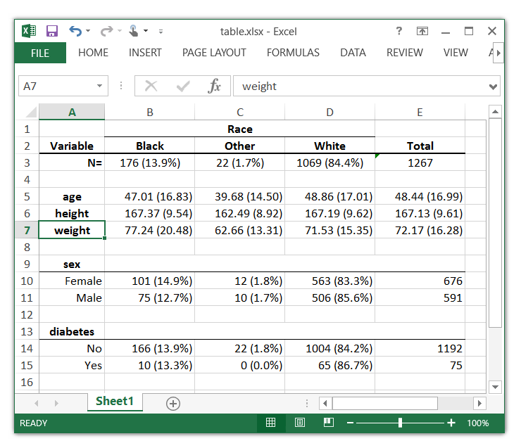
. ExcelTable race, cont(age height weight) cat(sex diabetes)
The Excel table table.xlsx was created successfully

and get an Excel table that looks like this:

So I wrote a program called ExcelTable for my own use Read more…

In this blog post, I’d like to give you a relatively nontechnical introduction to Markov chain Monte Carlo, often shortened to “MCMC”. MCMC is frequently used for fitting Bayesian statistical models. There are different variations of MCMC, and I’m going to focus on the Metropolis–Hastings (M–H) algorithm. In the interest of brevity, I’m going to omit some details, and I strongly encourage you to read the [BAYES] manual before using MCMC in practice.

Let’s continue with the coin toss example from my previous post Introduction to Bayesian statistics, part 1: The basic concepts. We are interested in the posterior distribution of the parameter \(\theta\), which is the probability that a coin toss results in “heads”. Our prior distribution is a flat, uninformative beta distribution with parameters 1 and 1. And we will use a binomial likelihood function to quantify the data from our experiment, which resulted in 4 heads out of 10 tosses. Read more…

In this blog post, I’d like to give you a relatively nontechnical introduction to Bayesian statistics. The Bayesian approach to statistics has become increasingly popular, and you can fit Bayesian models using the bayesmh command in Stata. This blog entry will provide a brief introduction to the concepts and jargon of Bayesian statistics and the bayesmh syntax. In my next post, I will introduce the basics of Markov chain Monte Carlo (MCMC) using the Metropolis–Hastings algorithm. Read more…

This post was written jointly with David Drukker, Director of Econometrics, StataCorp.

In our last post, we introduced the concept of treatment effects and demonstrated four of the treatment-effects estimators that were introduced in Stata 13.  Today, we will talk about two more treatment-effects estimators that use matching. Read more…

This post was written jointly with David Drukker, Director of Econometrics, StataCorp.

The topic for today is the treatment-effects features in Stata.

Treatment-effects estimators estimate the causal effect of a treatment on an outcome based on observational data.

In today’s posting, we will discuss four treatment-effects estimators:

1. RA: Regression adjustment
2. IPW: Inverse probability weighting
3. IPWRA: Inverse probability weighting with regression adjustment
4. AIPW: Augmented inverse probability weighting

We’ll save the matching estimators for part 2.

We should note that nothing about treatment-effects estimators magically extracts causal relationships. As with any regression analysis of observational data, the causal interpretation must be based on a reasonable underlying scientific rationale. Read more…

I was recently talking with my friend Rebecca about simulating multilevel data, and she asked me if I would show her some examples. It occurred to me that many of you might also like to see some examples, so I decided to post them to the Stata Blog. Read more…

Introduction

Today I want to show you how to create animated graphics using Stata. It’s easier than you might expect and you can use animated graphics to illustrate concepts that would be challenging to illustrate with static graphs. In addition to Stata, you will need a video editing program but don’t be concerned if you don’t have one. At the 2012 UK Stata User Group Meeting Robert Grant demonstrated how to create animated graphics from within Stata using a free software program called FFmpeg. I will show you how I create my animated graphs using Camtasia and how Robert creates his using FFmpeg. Read more…

Today I want to talk about effect sizes such as Cohen’s d, Hedges’s g, Glass’s Δ, η², and ω². Effects sizes concern rescaling parameter estimates to make them easier to interpret, especially in terms of practical significance.

Many researchers in psychology and education advocate reporting of effect sizes, professional organizations such as the American Psychological Association (APA) and the American Educational Research Association (AERA) strongly recommend their reporting, and professional journals such as the Journal of Experimental Psychology: Applied and Educational and Psychological Measurement require that they be reported. Read more…

What is it about round numbers that compels us to pause and reflect? We celebrate 20-year school reunions, 25-year wedding anniversaries, 50th birthdays and other similar milestones. I don’t know the answer but the Stata YouTube Channel recently passed several milestones – more than 1500 subscribers, over 50,000 video views and it was launched six months ago. We felt the need for a small celebration to mark the occasion, and I thought that I would give you a brief update.

I could tell you about re-recording the original 24 videos with a larger font to make them easier to read. I could tell you about the hardware and software that we use to record them including our experiments with various condenser and dynamic microphones. I could share quotes from some of the nice messages we’ve received. But I think it would be more fun to talk about….you!

YouTube collects data about the number of views each video receives as well as summary data about who, what, when, where, and how you are watching them. There is no need to be concerned about your privacy; there are no personal identifiers of any kind associated with these data. But the summary data are interesting, and I thought it might be fun to share some of the data with you. Read more…

In my last posting, I introduced you to the concepts of hierarchical or “multilevel” data. In today’s post, I’d like to show you how to use multilevel modeling techniques to analyse longitudinal data with Stata’s xtmixed command. Read more…