I care about reproducible research. Anyone who has ever been a research assistant or tried to follow the path set by other researchers also cares. Sometimes, reproducing others’ results is a frustrating task; sometimes, it is outright impossible. Yet sometimes, it is satisfyingly simple. In my experience, reproducing results is easy when it involves a Stata do-file. I believe this is true even beyond my personal bias (I work for Stata and used the software regularly before that). A recent article published by the American Economic Association (AEA), Vilhuber, Turrito, and Welch (2020), shows that Stata is the preferred package among economists, and I believe reproducibility is a big reason why. Read more…
The video below shows the cumulative number of COVID-19 cases per 100,000 population for each county in the United States from January 22, 2020, through April 5, 2020. The map doesn’t change much until mid-March, when the virus starts to spread faster. Then, we can see when and where people are being infected. You can click on the “Play” icon on the video to play it and click on the icon on the bottom right to view the video in full-screen mode.
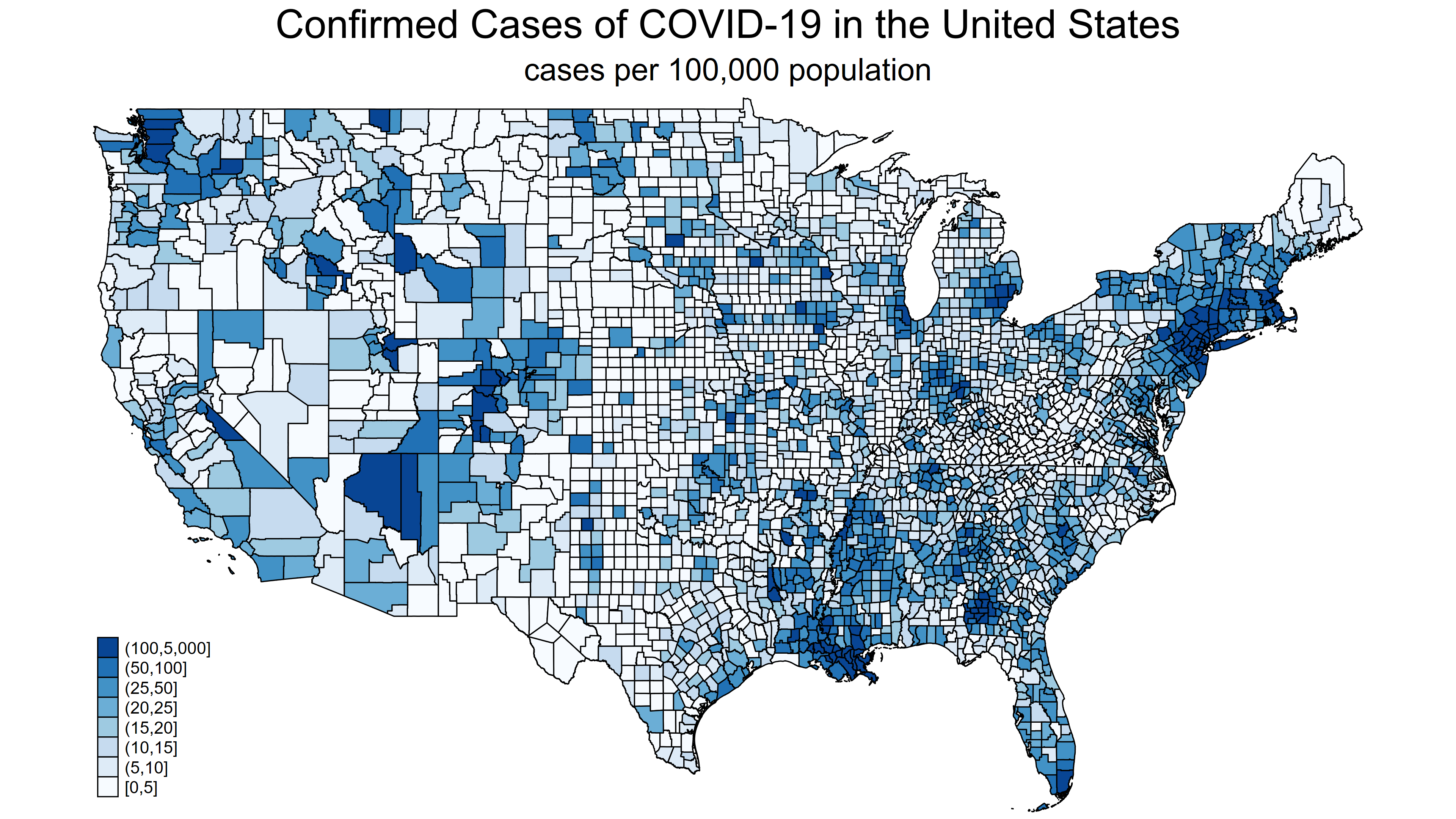
In my last post, we learned how to import the raw COVID-19 data from the Johns Hopkins GitHub repository and convert the raw data to time-series data. This post will demonstrate how to download raw data and create choropleth maps like figure 1.
Figure 1: Confirmed COVID-19 cases in United States adjusted for population size
In my last post, we learned how to import the raw COVID-19 data from the Johns Hopkins GitHub repository. This post will demonstrate how to convert the raw data to time-series data. We’ll also create some tables and graphs along the way. Read more…
In my last post, I mentioned that I did not want to distribute my covid19.ado file because “it could be rendered useless if or when Johns Hopkins changes its data”. I wrote that on March 19, 2020, and the data changed on March 23, 2020. This will likely happen again (and again, and again …). I may post updates in the future as the data change, but you may need to adapt sooner than I can post. So let’s see how we can update our code to adapt to the changing data. Read more…
Like many of you, I am working from home and checking the latest news on COVID-19 frequently. I see a lot of numbers and graphs, so I looked around for the “official data”. One of the best data sources I have found is at the GitHub website for Johns Hopkins Whiting School of Engineering Center for Systems Science and Engineering. The data for each day are stored in a separate file, so I wrote a little Stata command called covid19 to download, combine, save, and graph these data. Read more…
Stata Press is pleased to announce the release of Introduction to Time Series Using Stata, Revised Edition, by Sean Becketti. This edition has been updated for Stata 16 and is available in paperback, eBook, and Kindle format. In this book, Becketti introduces time-series techniques—from simple to complex—and explains how to implement them using Stata. The many worked examples, concise explanations that focus on intuition, and useful tips based on the author’s experience make the book insightful for students, academic researchers, and practitioners in industry and government. Read more…
Markov chain Monte Carlo (MCMC) is the principal tool for performing Bayesian inference. MCMC is a stochastic procedure that utilizes Markov chains simulated from the posterior distribution of model parameters to compute posterior summaries and make predictions. Given its stochastic nature and dependence on initial values, verifying Markov chain convergence can be difficult—visual inspection of the trace and autocorrelation plots are often used. A more formal method for checking convergence relies on simulating and comparing results from multiple Markov chains; see, for example, Gelman and Rubin (1992) and Gelman et al. (2013). Using multiple chains, rather than a single chain, makes diagnosing convergence easier.
As of Stata 16, bayesmh and its bayes prefix commands support a new option, nchains(), for simulating multiple Markov chains. There is also a new convergence diagnostic command, bayesstats grubin. All Bayesian postestimation commands now support multiple chains. In this blog post, I show you how to check MCMC convergence and improve your Bayesian inference using multiple chains through a series of examples. I also show you how to speed up your sampling by running multiple Markov chains in parallel. Read more…
Sometimes, I like to augment a time-series graph with shading that indicates periods of recession. In this post, I will show you a simple way to add recession shading to graphs using data provided by import fred. This post also demostrates how to build a complex graph in Stata, beginning with the basic pieces and finishing with a polished product.
The holidays are fast approaching, and if you’re like most people, you’re still not exactly sure what gift or gifts to get those special people in your life. Enter the Stata Certified Gift Guide. We polled our team and compiled their favorites into the ultimate gift guide for data lovers! Sure, you could go the typical gift card route, but where’s the fun in that?
Power Nap Pillow $99.00
Sometimes, you just need to close the door and take a power nap.